Category: ML

  • MSD0034 RAG Customer Support Assistant

    Design a RAG-based customer support assistant for a company like Stripe, Shopify, or a large telecom. The assistant is grounded in the company’s own knowledge base: help articles, product documentation, past resolved tickets, and policy pages. It must answer accurately, cite its sources, refuse to fabricate when the answer is not in the knowledge base, escalate to a human when the question is high-stakes (billing, account access, legal) or when its confidence is low, and stay current as the knowledge base is edited every day.

    The cost structure is asymmetric: a hallucinated refund policy or a confident wrong answer about account access is far worse than admitting ignorance and handing the conversation to an agent. A wrong answer can create a chargeback, a regulatory complaint, or a churned account, while an escalation costs a few dollars of agent time.

    How would you design this system? Cover the retrieval architecture (chunking, embedding, hybrid search, re-ranking), the generation and grounding strategy, the confidence and safety gating that decides when to answer versus escalate, the human handoff path with full context, and how you evaluate answer quality and hallucination rate.

    Line-art scene: a customer asking about a refund window, a knowledge base of help articles and resolved tickets, a question mark, and a warning that a confident wrong policy costs more than admitting ignorance

    The Problem: the answer either exists somewhere in a knowledge base that changes daily, or it does not exist at all, and the system has to tell those two cases apart before it opens its mouth.

    Answer

    The design is a retrieve, re-rank, generate pipeline wrapped in an explicit answer policy. Hybrid retrieval over structure-aware chunks pulls 50 candidates, a cross-encoder re-ranker trims them to 8, and the generator may only assert what a cited passage actually says. Two decisions carry the answer. First, abstention and escalation are first-class outputs: a risk classifier runs before generation, a retrieval-confidence threshold guards coverage, and a per-claim groundedness verifier checks the draft, so the default under doubt is a warm human handoff rather than a fluent guess. Second, the index is versioned and refreshed nightly by delta, with product, plan, and region metadata as hard filters, because most support “hallucinations” are really retrieval of the wrong but plausible policy version.

    (1) Structure-Aware Chunking: split on headings at roughly 400 tokens with 15% overlap, keep tables and code blocks intact, and prepend the article title and breadcrumb so an isolated chunk is self-describing.
    (2) Rich Chunk Metadata: product, plan, region, locale, source type, version, and effective date travel with every chunk and act as hard filters before scoring.
    (3) Hybrid Retrieval Plus Re-ranking: BM25 catches error codes, SKUs, and API field names; dense embeddings catch paraphrase; fusion gives 50 candidates and a cross-encoder picks the top 8.
    (4) Citation-Constrained Generation: numbered passages in the prompt, sentence-level citation ids in a structured output, low temperature, and an explicit insufficient_context abstain option.
    (5) Three-Gate Answer Policy: risk classifier, retrieval-confidence threshold, and claim-level groundedness check; any gate that fires routes to a human instead of shipping the text.
    (6) Warm Handoff and Content Loop: the agent inherits the transcript, the exact passages used, the extracted entities, and a draft reply; the agent’s final answer becomes an eval label and, when the gap is real, a new article.

    RAG support pipeline: user question and session context flow into query rewrite with a risk classifier, hybrid retrieval, cross-encoder re-ranking, grounded generation with citations, then an answer gate that either sends a cited answer or hands off to a human agent with context

    Figure 1: One pass per question: rewrite and risk-classify, retrieve and re-rank, generate only from the surviving passages, then let the gate decide whether the customer sees the text or an agent does.

    Clarify Before Designing:
    (1) Volume and Channels: how many chat sessions per day, how many turns each, which languages, and is the user authenticated when they ask?
    (2) Quality Bar and Deflection Target: what accuracy floor must hold for answers we do give, and who signs off on the refusal rate that buys it?
    (3) Knowledge Base State: how much content is written for customers versus internal agents, are policies versioned by region and plan, and are ticket resolutions quality-reviewed?
    (4) Account Access: may the assistant read account state (plan, invoices, outage status) through tools, or only public docs? This changes both retrieval and the risk gate.
    (5) Latency and Cost Budget: target first token, target full answer, and the per-conversation cost ceiling relative to an agent contact.
    (6) High-Stakes Definition: which intents are legally or financially sensitive (billing disputes, cancellation, identity, data deletion) and what retention rules apply to logged conversations?


    Login to view more content
  • MSD0033 Drowsy Driving Detection

    Design a drowsy-driving detection system that uses an in-car camera to monitor the driver and warn before they fall asleep, as offered by Volvo’s Driver Alert, Mercedes Attention Assist, and aftermarket dashcam apps. The system must run on an embedded device or a phone mounted on the dashboard, process the camera feed in real time, and detect early signs of drowsiness (eyelid closure duration, blink rate, head nodding, gaze wandering, micro-sleeps) with few false alarms so drivers do not disable it. It must work across drivers of different appearance, in varying lighting (night, tunnels, sunglasses), and it must keep the video on-device.

    How would you design this system? Cover the face and landmark detection, the drowsiness signal extraction (PERCLOS, blink dynamics, head pose), the temporal model that combines signals over a window, the on-device deployment and privacy design, and how you calibrate the alert threshold to minimize false alarms without missing real drowsiness.

    Line-art scene: a driver behind the steering wheel with closing eyelids, a dashboard camera watching, and a timeline of four eye states from open to micro-sleep with a question mark over the moment the warning should fire

    The Problem: the dangerous state lasts a few seconds and arrives after minutes of visible warning signs, so the system has to fire during the slow decline, at night, through sunglasses, and almost never on an alert driver.

    Answer

    The design is a landmark-driven feature pipeline with a learned temporal model: a cheap face detector runs on a fraction of frames with a tracker in between, a landmark network gives eye, mouth, and head-pose geometry per frame, hand-designed physiological features (PERCLOS, blink dynamics, nod and gaze statistics) are accumulated over a sliding 60-second window, and a small recurrent model maps that window to a drowsiness score. The two pivotal decisions are to keep interpretable intermediate signals rather than regressing drowsiness end-to-end from pixels, and to treat the alert threshold as a calibrated operating point on a false-alarms-per-hour axis with hysteresis, because a system that chirps at an awake driver gets unplugged on day two. Everything runs on-device on an int8 quantized graph with a near-infrared sensor, and no frame is ever written to storage or uploaded.

    (1) Geometric Landmark Pipeline: face detection plus a landmark network feeding eye aspect ratio, PERCLOS, blink timing, and head pose; features are physiologically interpretable and cheap.
    (2) End-to-End Video Model: a 3D CNN or video transformer over eye-region crops predicting drowsiness directly, learning subtle cues no geometric feature encodes, at a much higher data and compute cost.
    (3) Hybrid Fusion (chosen): geometric features per frame plus a small GRU over the 60-second window, with per-driver normalization and hysteresis on the output score.
    (4) Vehicle-Signal Baseline: steering entropy, lane-position variance, and pedal behavior with no camera at all, which is what Volvo’s original Driver Alert used; it is robust to lighting but needs minutes of degraded driving before it reacts.

    Three-row mechanism diagram: camera, amortized face detector, landmark network and per-driver normalization on top; PERCLOS, blink dynamics and head pose plus gaze signals in the middle; temporal GRU fusion, score with hysteresis and escalating alert at the bottom, all on-device

    Figure 1: Per-frame geometry becomes per-window physiology, and only the last stage makes a decision: pixels never leave the device and never leave RAM.

    Clarify Before Designing:
    (1) Sensor: RGB rolling-shutter phone camera or a dedicated near-infrared global-shutter module with an 850 nm illuminator, and at what resolution and frame rate?
    (2) Compute Target: a phone with an NPU delegate, an automotive SoC, or a low-power MCU, and what sustained thermal and power budget do we get on a 4-hour drive?
    (3) Alert Budget: how many false alarms per driving hour before drivers disable the feature, and are we targeting a regulated warning profile (UNECE ADDW-style) or a comfort feature?
    (4) Labels: do we have annotated drowsy driving data with KSS self-reports or expert video scoring, and how many distinct drivers, or only simulator and public sets?
    (5) Occlusion Requirements: must the system work through sunglasses and face masks, or may it declare “sensing unavailable” and fall back to vehicle signals?
    (6) Action Space: what can the alert actually do (chime, haptic seat or wheel, escalating voice prompt, rest-stop suggestion), since the escalation ladder shapes the threshold.


    Login to view more content
  • MSD0032 End-to-End Self-Driving

    Design an end-to-end learning model for self-driving, where a single neural network (or a tightly coupled stack) maps raw sensor inputs directly to driving actions (steering, acceleration, braking), as pursued by Tesla’s FSD v12+, Wayve’s LINGO, and research systems like UniAD and VAD. Unlike the traditional modular pipeline of separate perception, prediction, planning, and control modules, an end-to-end model learns the full policy from data and can in principle optimize the driving objective globally.

    The catch is that this policy is a black box. It is hard to interpret, hard to verify for safety, hungry for data and compute, and it only ever sees the long tail of rare driving situations a handful of times.

    How would you design this model? Cover the candidate architecture approaches (pure end-to-end policy network vs loosely coupled perception-prediction-planning with learned interfaces vs hybrid with a differentiable cost head), the training data and objective (imitation learning vs reinforcement learning vs inverse RL), how you handle the long tail of rare safety-critical events when learning from data, and how you verify and debug a black-box policy before deployment.

    Line-art scene: camera and ego-state boxes feed a question-mark box that outputs steering and pedal commands, above a long road arrow whose dense head markers are common events and whose sparse tail markers are rare events under a magnifier

    The Problem: one learned function must turn photons into pedal and steering commands, and the events that decide whether it is safe appear once every hundred thousand miles.

    Answer

    I would build a query-based end-to-end network with a differentiable cost head, not a raw pixels-to-pedal regressor. Multi-camera features are lifted into a BEV representation, a set of scene queries carries agents, map, and occupancy, and an ego query cross-attends to those queries to produce a short-horizon trajectory that a learned cost head scores together with a few hand-authored terms. Everything is trained jointly with one driving loss, so gradients still reach the encoder, but every intermediate is supervised and therefore inspectable. The two pivotal decisions are to keep auxiliary supervision on the intermediate queries (this is what buys sample efficiency and debuggability without cutting the gradient path) and to keep hard safety constraints outside the learned cost, in an independent rule-based guardian that the network cannot argue with.

    (1) Pure End-to-End Policy: one network maps sensor history directly to control, trained by behavior cloning on fleet data with no intermediate supervision.
    (2) Loosely Coupled Modules with Learned Interfaces: perception → prediction → planning stays as stages, but the interfaces are differentiable query tokens rather than hand-defined object lists, as in UniAD and VAD.
    (3) Hybrid with a Differentiable Cost Head: the network emits a learned cost over candidate ego trajectories, combined with explicit collision, comfort, and rule terms, and an optimizer or sampler picks the executed trajectory.
    (4) Chosen Combination: approach 2 for the representation plus approach 3 for the output, imitation pretraining followed by closed-loop fine-tuning in simulation.

    Architecture diagram: sensors feed a BEV encoder, then scene queries for agents, map and occupancy, then an ego planner head, then a trajectory and control output; auxiliary supervision hangs below the encoder and queries, and a differentiable cost head sits below the planner

    Figure 1: The chosen architecture. One driving loss backpropagates all the way to the encoder, while auxiliary heads keep the intermediate scene representation readable and the cost head keeps the final decision expressible in physical terms.

    Clarify Before Designing:
    (1) Sensor Suite And Output Interface: camera-only or camera plus lidar and radar, and does the model emit a 3 second trajectory for a downstream controller or raw actuator commands?
    (2) Compute And Latency Budget: how many TOPS on-vehicle and what reaction budget, since that caps token count, temporal context, and model size?
    (3) Data Access: fleet miles per day, whether human control signals are time-aligned with sensors, and whether a closed-loop simulator with reactive agents exists.
    (4) Operational Design Domain: highway lane keeping, dense urban, or both, and in which geographies and weather, because the ODD size sets the length of the tail.
    (5) Safety Architecture: is an independent rule-based guardian or a safety driver allowed downstream, or must the network’s output be the last word before the actuators?


    Login to view more content
  • MSD0031 Autonomous Sensor Fusion

    Design the sensor fusion system for an autonomous vehicle that combines camera, LiDAR, and radar into a unified perception of the world, as used by Waymo, Cruise, and Tesla’s Full Self-Driving stack. Each sensor has complementary strengths (camera: dense semantic and color detail; LiDAR: accurate depth and 3D structure; radar: velocity and all-weather range) and weaknesses (camera: depth ambiguity and weather sensitivity; LiDAR: sparse, expensive, poor in fog and rain; radar: low angular resolution and clutter). The fused perception must feed detection, tracking, and prediction at 10-20 Hz with hard latency bounds, and it must degrade gracefully when a sensor fails or is occluded rather than producing a confident wrong answer.

    How would you design this system? Cover the per-sensor processing, the fusion architecture (early, late, or mid-level BEV fusion), the time synchronization and calibration, how you handle sensor dropout and degradation, and how you evaluate fusion quality against single-sensor baselines.

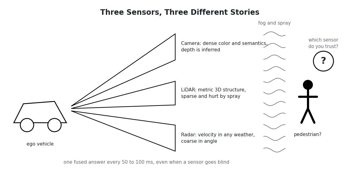
    Line-art scene: an ego vehicle emitting three sensor beams labeled camera, LiDAR, and radar toward a pedestrian half-hidden in fog and road spray, with a question mark asking which sensor to trust

    The Problem: three sensors look at the same road spray and return three different stories, and the vehicle still has to emit one confident answer every 50 to 100 ms.

    Answer

    Build a mid-level fusion stack over a shared bird’s-eye-view (BEV) grid. Each sensor keeps its own encoder, every feature is warped into one metric grid at one reference timestamp, and a lightweight transformer fuses them before the detection, occupancy, and tracking heads. Mid-level fusion is the pivotal choice: early raw fusion is brittle under calibration drift and blocks per-sensor pretraining, while late fusion discards exactly the cross-modal evidence that resolves camera depth ambiguity and rescues weak single-sensor detections. Two further decisions carry the safety argument. Train with modality dropout so the fused model remains usable when a sensor disappears, and keep a small non-learned geometric path (radar Doppler tracks plus LiDAR clustering) that can hold the vehicle to a safe stop if the learned stack degrades.

    (1) Shared BEV Representation: project all modalities into a common ego-centric grid (roughly 100 m by 100 m at 0.4 m resolution) so fusion is a geometric alignment problem rather than an ad hoc feature concatenation.
    (2) Per-Sensor Encoders: depth-distribution lift for images, sparse voxel or pillar encoder for LiDAR, and a point encoder that keeps radar range-rate; each branch trains and validates independently.
    (3) Soft-Association Fusion: cross-attention between object queries and per-sensor features instead of hard pixel-to-point matching, which keeps accuracy when extrinsics drift by a fraction of a degree.
    (4) Hardware Sync and Online Calibration: PTP-locked triggers, per-point timestamps, and ego-motion warping to one reference time, with reprojection residuals monitored continuously as a calibration health signal.
    (5) Fallback Ladder: a health monitor scores each sensor and steps the system from full fusion, to degraded fusion with widened safety margins, to the geometric path plus an ODD exit or minimal risk maneuver.
    (6) Ablation-Gated Evaluation: the release rule is that fused perception is never worse than the best single-sensor baseline on any evaluation slice, including night, rain, and forced-dropout slices.

    Fusion pipeline: cameras, LiDAR, and radar feed a time-sync and calibration stage, then per-sensor encoders, a BEV fusion transformer, and detection, occupancy, and tracking heads, with a sensor health monitor feeding a geometric fallback path into tracking

    Figure 1: One learned path through a shared BEV grid, plus a health monitor and a non-learned geometric path that stays alive when the learned path should not be trusted.

    Clarify Before Designing:
    (1) Sensor Suite and Cost Ceiling: how many cameras, what LiDAR (spinning 64-beam, solid state, or none), how many radars, and is 4D imaging radar available?
    (2) Operational Design Domain: geofenced urban robotaxi with HD maps, or consumer highway assist without maps; does the ODD include heavy rain, snow, and night?
    (3) Compute and Latency Budget: on-vehicle TOPS, power and thermal envelope, target rate (10 Hz or 20 Hz), and the p99 rather than mean latency bound.
    (4) Failure Policy: on sensor loss, does the vehicle degrade speed, exit the ODD, hand back to a driver, or execute a minimal risk maneuver; who signs off on that decision?
    (5) Label Supply: how much human-labeled 3D data exists, and can an offboard auto-labeling pipeline produce pseudo ground truth from full logs?
    (6) Redundancy Requirement: must perception survive the loss of any single sensor, or any single compute unit, and is a second independent stack mandated?


    Login to view more content
  • MSD0030 Google Maps Traffic Prediction

    Design the traffic prediction system behind Google Maps’ ETA and route recommendations. The system must forecast road speeds and congestion on every segment of a global road network, minutes to hours ahead, so that routing can pick the fastest path and display accurate arrival times.

    It must fuse real-time probe data from millions of phones and fleet vehicles, historical patterns, live incidents (accidents, construction, events), and weather. It also has to respect the spatial and temporal dependencies that make a jam on one freeway cascade onto adjacent arterials minutes later.

    How would you design this system? Cover the data ingestion and map-matching pipeline, the spatio-temporal forecasting model, how real-time and historical signals are combined, how incidents and events are incorporated, and how the ETA is computed and kept honest as conditions change.

    Line-art scene: a congested freeway spilling traffic onto side streets, phones sending probe pings upward, and a clock with a question mark asking what arrival time to promise

    The Problem: a jam does not stay on one road and probe coverage is uneven, yet the product must commit to a single arrival time for every trip, everywhere, right now.

    Answer

    The design is a streaming pipeline that turns anonymized probe traces into per-segment speed observations, then a spatio-temporal graph neural network over the road network that predicts a multi-horizon quantile speed distribution for every segment. Predictions are precomputed into a distributed speed store, and the routing engine reads them as time-dependent edge weights, so a route query never waits on a model call. Two decisions are pivotal. First, the model operates on supersegments (chains of consecutive segments that share traffic) rather than isolated edges, which fixes probe sparsity and lets message passing carry a jam upstream and onto parallel arterials. Second, the real-time signal is a residual on top of a historical speed profile, not a replacement for it, so accuracy degrades gracefully as probe density drops and as the horizon grows. Google’s published version of this system reports ETA accuracy improvements of up to 50% in several metros after moving from segment-local models to a GNN over supersegments.

    (1) Map Matching And Aggregation: HMM map matching snaps noisy GPS traces to road segments, and traversals are aggregated into short time bins per segment and supersegment so no individual trip is recoverable.
    (2) Historical Prior Plus Live Residual: a per-segment, per-time-of-week speed profile is the baseline; the live signal predicts the deviation from it, which is what makes sparse-probe roads survivable.
    (3) Spatio-Temporal GNN: nodes are segments with live, historical, and static features; two to three rounds of message passing propagate congestion along the network, and multi-horizon heads emit speeds at 2, 10, 30, and 60 minutes.
    (4) Incidents As Features Plus A Short-Horizon Override: accidents, closures, events, and weather enter as node and context features, with a corroborated override path that patches the next few minutes faster than the model can retrain.
    (5) Precompute And Serve: predictions land in a segment-by-horizon key-value store read in single-digit milliseconds; routing runs time-dependent search so long trips use future speeds, not present ones.
    (6) Quantile ETA And Mid-Trip Correction: the product shows a calibrated interval rather than a point estimate, and the ETA is re-estimated during the trip as the vehicle’s own trace becomes evidence.

    Traffic prediction pipeline: probe streams flow into HMM map matching and aggregation, a spatio-temporal GNN produces multi-horizon quantile speeds, results are written to a speed store read by time-dependent routing, with a feature store of history, incidents and weather feeding the model and realized travel times feeding retraining

    Figure 1: The serving path: probes become segment observations, the model writes future speeds ahead of time, and the router only reads. Realized travel times close the loop as training labels.

    Clarify Before Designing:
    (1) Coverage And Probe Density: which markets, and what fraction of segments see enough probes in a five-minute window to support a live estimate at all?
    (2) Horizon And Refresh: do we only serve depart-now ETAs, or also scheduled departures hours ahead, and how often must each segment be refreshed?
    (3) Latency Budget: what is the end-to-end budget for a route query, and is the prediction allowed to run inline or must it be precomputed?
    (4) Error Asymmetry: is arriving late worse than arriving early, and by how much, since that decides which quantile we display?
    (5) Privacy Constraints: what aggregation thresholds and retention limits apply to location traces, and do they differ by region?
    (6) Routing Ownership: do we control the routing engine (so we can change edge weights and spread traffic) or only publish speeds to a consumer?


    Login to view more content
  • MSD0029 Food Calorie Estimation

    Design a model that estimates the calorie and macronutrient content of a meal from a single photo, as used by apps like MyFitnessPal, Calorie Mama, or Lose It. The user snaps a photo of their plate. The model must identify the dishes, estimate portion sizes from a 2D image with no depth cue, look up or predict per-gram nutritional values, and return a calorie estimate within a few seconds.

    The core technical challenge is portion estimation: a single 2D photo carries no metric depth, so converting pixel area into grams requires a mechanism assumption. The model must also handle a long tail of cuisines and homemade dishes that match no packaged-food database, varying plating and lighting, and the inherent ambiguity of judging a portion from one viewpoint.

    How would you design this model? Cover the candidate portion estimation approaches (monocular depth estimation, reference-object scaling, semantic segmentation with food-class density priors, and direct end-to-end calorie regression), how you handle the long tail of homemade and mixed dishes, how you generate training labels at scale when ground-truth portion weights are scarce, and how you calibrate and communicate uncertainty when a single 2D photo is inherently ambiguous.

    Line-art scene: a phone photographs a plate top-down, and two unseen side views with identical pixel area show a flat serving of about 120 g and a mounded serving of about 380 g, with a question mark between them

    The Problem: the same mask area can be a thin layer or a tall mound, so one photo maps to a wide range of grams before any model has made a single assumption explicit.

    Answer

    The design is a segmentation-conditioned multi-task regressor. One shared backbone emits per-dish instance masks, a relative depth map, and a direct per-region regression of grams, calories, and macronutrients, with the physical volume-times-density estimate retained as a parallel sanity check rather than as the primary predictor. Google’s Nutrition5k study drives that ordering: an end-to-end regressor from a single RGB view reaches roughly 26% mean calorie error, and feeding depth — either as an extra channel or as a depth-derived volume scalar — cuts that error substantially, which is why depth is an auxiliary input to the regressor here rather than the front end of a separate segment-then-volume-then-density-lookup chain. Two decisions are pivotal. First, scale is treated as a learned prior anchored by plate and utensil geometry, not as metric information that a single RGB frame secretly contains. Second, the output is a calibrated interval and an editable suggestion, because one viewpoint leaves real ambiguity that no architecture removes.

    (1) Monocular Depth Volume: predict per-pixel depth, fit the plate plane, and integrate height over each mask to get volume, then multiply by a food-class density. Physically interpretable, but scale-ambiguous.
    (2) Reference-Object Scaling: use a known-size object in frame (bank card, coin, thumb, standard plate rim) to fix millimeters per pixel in the plate plane, which pins down area but not height.
    (3) Segmentation With Density Priors: multiply mask area by a learned per-class height prior and a tabulated density in grams per cubic centimeter from food-composition data. Cheapest to build and to explain.
    (4) Direct End-to-End Regression: regress grams, kilocalories, and macros straight from region features, letting the network learn scale from plate, cutlery, and hand context. Most accurate where labels exist, least interpretable.

    Mechanism diagram: one photo enters a shared backbone that feeds an instance segmentation head, a metric depth head, and a per-region regression head; segmentation and depth feed a physical volume-times-density check, which is fused with the regression output through a conformal interval step into calories, macros, and a range

    Figure 1: The mechanism: photo → masks and depth → grams per dish, with the physical volume path acting as a guardrail on the learned regressor and a conformal step turning the point estimate into a range.

    Clarify Before Designing:
    (1) Label Ground Truth: do we have any scale-weighed dishes with per-ingredient masses, or only crowd labels and user-entered corrections?
    (2) Capture Protocol: is it strictly one top-down snap, or may we request an oblique angle, a second frame, or a reference object without destroying adoption?
    (3) Depth Sensors: what fraction of devices expose LiDAR or ARKit/ARCore depth, which turns scale from a guess into a measurement?
    (4) Accuracy Bar: what calorie error is product-acceptable, and does the UX accept a range plus an edit control instead of one number?
    (5) Coverage And Budget: which cuisines dominate traffic, what share of meals is packaged or restaurant food with known nutrition, and is inference on-device or server-side?


    Login to view more content
  • MSD0028 Deepfake AIGC Detection

    Design a deepfake and AI-generated content detection system for a video platform like YouTube or TikTok. Generative video models (Sora, Runway, Kling) and voice cloning tools have made convincing synthetic media cheap, and the platform must label or remove media that misleads viewers, impersonates real people, or spreads disinformation, while leaving legitimate creative and artistic uses of the same tools untouched.

    The detector has to keep up with generators that improve every few months, survive uploads that were re-encoded and re-compressed until most forensic cues are gone, and avoid flagging real content that merely looks synthetic (high-quality CGI, heavily graded or filtered footage, screen recordings).

    How would you design this system? Cover the detection signals (frequency artifacts, temporal inconsistencies, biometric cues, provenance metadata like C2PA), the model architecture for image, audio, and video, how you handle the adversarial arms race against improving generators, the human-review and appeals path, and how you measure detection rate and false-positive rate.

    Line-art scene: an upload funnel feeding three video frames (a real phone clip, an AI-generated clip under a magnifier, and a CGI shot) into a viewer's feed, with a question mark above the viewer

    The Problem: three clips reach the same viewer, one filmed, one generated, one hand-made CGI. Only the misleading one should be acted on, and the pixels have already been re-encoded to 480p before you ever see them.

    Answer

    The design is a provenance-first, harm-tiered cascade, not a binary “fake or real” classifier. Every upload is first checked for signed C2PA Content Credentials and invisible watermarks, then a cheap multimodal triage model scores sampled frames plus the audio track, and only the riskiest few percent enter a heavy visual, audio, and temporal ensemble. The two pivotal decisions are that the system outputs a calibrated risk score plus a harm class (impersonation of a real person, medical or election claim, synthetic-but-harmless art) which drives graduated enforcement rather than blanket removal, and that the whole training and evaluation loop is built around the arms race: continuous harvesting of every new generator family, red teaming, and a release gate measured on unseen-generator holdouts and in-the-wild data instead of academic benchmarks.

    (1) Provenance First, Detection Second: validate C2PA manifests and watermark decoders before any classifier runs; a valid signature is strong positive evidence, but a missing one proves nothing because metadata is stripped by every transcode.
    (2) Cheap Triage, Expensive Ensemble: a small model scores 100% of uploads, the deep ensemble runs on roughly 2%, keeping compute inside budget while preserving recall on the tail that matters.
    (3) Multimodal Signal Stack: spatial and frequency artifacts, temporal cues (landmark jitter, blink rate, rPPG pulse, lip-sync offset), and audio cues (vocoder phase artifacts) fused late, so no single fragile signal owns the decision.
    (4) Compression-Robust Training: synthetic training data is pushed through the platform’s own transcode ladder, because a detector trained on pristine generator output collapses on real uploads.
    (5) Harm-Tiered Enforcement: disclosure label, then demotion, then human review, then removal; full automation only for narrow high-confidence classes such as a cloned voice of a verified public figure.
    (6) Arms-Race Loop: a red team plus a generation farm produce fresh fakes from every new model release, feeding a 2 to 4 week retrain cadence with an emergency path.

    Detection pipeline: upload flows through provenance checks, cheap triage, a deep ensemble, and fusion into enforcement tiers, with human review and appeals feeding a training store that retrains the ensemble

    Figure 1: One cheap pass over everything, one expensive pass over the risky tail, and a review loop whose overturns become next week’s training data.

    Clarify Before Designing:
    (1) Policy Scope: are we labeling all synthetic media, or only synthetic media that misleads (impersonation, fabricated events, health and election claims)? The answer changes the target variable itself.
    (2) Scale and Latency: uploads per day and peak factor, and must a verdict land before publish or within minutes after, before the video can go viral?
    (3) Provenance Coverage: what fraction of uploads arrive with valid C2PA credentials or a decodable watermark today, and which camera and tool partners are signed up?
    (4) Ground Truth: do we have licensed API access to the major generators for in-house fake production, and how many human-confirmed in-the-wild labels per week does review produce?
    (5) Cost Asymmetry: what does a missed political deepfake cost versus a wrongly demoted VFX creator, and how large is the review headcount that sets our false-positive budget?
    (6) Jurisdiction: which transparency rules apply (EU AI Act disclosure duties, election-period rules), and do they force labels regardless of harm?


    Login to view more content
  • MSD0027 Fake Account Bot Detection

    Design a system to detect fake accounts and bots on a social network like Facebook, Twitter/X, or Instagram. Fake accounts power spam, coordinated inauthentic behavior, follower farming, and political manipulation, and their operators evolve constantly: they buy aged accounts with real history, use LLMs to write bios and mimic human posting cadence, and route traffic through residential proxies so IP reputation says nothing.

    The system must score accounts at creation time and keep re-evaluating them as behavior develops, while holding the false-positive rate low enough that real users are not wrongly suspended, and routing the highest-risk cases to human investigators.

    How would you design this system? Cover the account-level feature signals (registration, graph, content, behavior), the detection model architecture, how you handle adversarial evolution, the human-in-the-loop review queue, and how you measure precision and recall when ground truth is scarce.

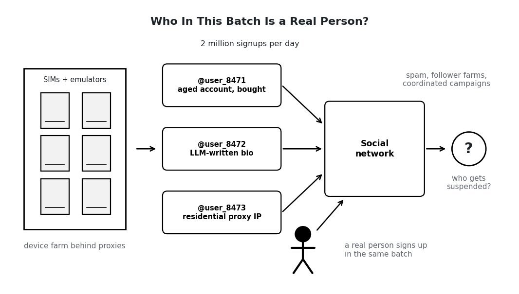
    Line-art scene: a device farm of phones behind a proxy feeds a stack of new account cards into a social network, with a real person in the same batch and a question mark asking who is fake

    The Problem: millions of new accounts a day, a farm that can forge everything cheap to forge, and one real person sitting in the same batch. Decide who to trust without suspending them.

    Answer

    Treat this as two coupled problems running at two speeds. At signup, a low-latency gradient-boosted scorer over registration, device, and infrastructure features decides whether the account starts with friction, and a continuous re-scoring layer then re-judges every live account as its graph and behavior accumulate. That second layer is where the real detections happen: a relational GNN over the follow and friend graph plus unsupervised synchrony clustering (the SynchroTrap idea of co-clustering accounts that act on the same targets in the same time buckets) catches campaigns whose individual members each look perfectly human. Scores never map directly to bans. They map to a graduated enforcement ladder (allow, challenge, limit reach, human review, disable) so the expensive mistake, suspending a real user, requires either overwhelming cluster-level evidence or an investigator.

    (1) Two-Speed Detection: a synchronous per-signup scorer under a 200 ms budget, plus a daily (and event-triggered) batch pass over every active account, since most fake accounts only reveal themselves after they start acting.
    (2) Cluster-Level Evidence: the decision unit is the account and the campaign; graph plus action-synchrony clustering finds coordinated groups without needing labels for the new tactic.
    (3) Cost-To-Forge Feature Weighting: prefer signals an operator must pay real money or real time to fake (device integrity, aged organic graph, human-only interaction telemetry) over signals a proxy or an LLM erases for free.
    (4) Graduated Enforcement: friction first (phone or CAPTCHA challenge, reach limiting), auto-disable only in the top band with corroboration, always with an appeal path that feeds labels back.
    (5) Label Machinery: reviewer verdicts, appeal reversals, honeypot and test-buy cohorts, and a random-audit stream, because production has no clean ground truth and the flagged sample alone teaches the model its own blind spots.

    Pipeline: signup and live accounts feed a feature store, which serves a fast GBDT scorer and a daily graph and synchrony pass; a policy engine maps scores to allow, challenge or limit, or a human review queue, whose verdicts flow to a label store and weekly retraining

    Figure 1: Two speeds, one policy: a synchronous scorer at signup, a daily graph and synchrony pass over every live account, and a ladder whose top band ends at a human, not a model.

    Clarify Before Designing:
    (1) Scale And Prevalence: how many signups per day, how many active accounts to re-score, and what does the current prevalence estimate say (a few percent of MAU)?
    (2) False-Positive Budget: how many wrongly restricted real users per day is the product willing to accept, and is auto-suspension allowed at all under the platform’s appeal and regulatory commitments?
    (3) Enforcement Surface: can we impose signup friction (phone verification, CAPTCHA), or does growth own that decision and force us to detect after the fact?
    (4) Review Capacity: how many investigator-hours per day exist, in which languages and regions, and what is the target queue latency for high-harm cases?
    (5) Threat Priority: which abuse type pays first, follower farms, spam, or coordinated political campaigns, since they differ in scale, sophistication, and tolerance for delay?
    (6) Signal Access: what device, telemetry, and payment signals are legally usable per region, and how long may we retain them?


    Login to view more content
  • MSD0026 Multimodal Text-to-Image-Video Search

    Design a multimodal search system where a user types a text query and the system returns relevant items from a catalog of billions of images and videos, like Pinterest Visual Search, Google Lens, or TikTok’s visual search. The query may describe objects, scenes, styles, or actions that never appear as literal text anywhere in the catalog (for example “golden retriever catching a frisbee at sunset”), so the system must bridge the modality gap between language and visual content.

    Results must return in under 200 ms, the index must stay fresh as new content is uploaded continuously, and the system must handle queries that mix text with an uploaded reference image.

    How would you design this system? Cover the shared embedding space and training strategy, the approximate nearest neighbor index at billion scale, the freshness and update strategy, the hybrid text-plus-image query path, and how you evaluate retrieval quality.

    Line-art scene: a person typing a descriptive sentence into a search box on the left, a dashed divide with a question mark in the middle, and a grid of image and video tiles representing billions of catalog items on the right

    The Problem: the words the user types appear nowhere in the catalog, yet the right pixels have to surface out of billions of items inside 200 ms, while new uploads keep arriving.

    Answer

    The design is a two-tower (dual encoder) retrieval system over one shared embedding space, served as a two-stage retrieve-and-rerank path. A contrastive image-text model of the SigLIP/CLIP family, fine-tuned on in-domain query-engagement pairs, maps text, images, and video clips into the same 512-d space, so “golden retriever catching a frisbee at sunset” becomes a vector whose neighbors are the right pixels even though no matching caption exists. Two decisions carry most of the weight. First, the item side is multi-vector for video (a handful of clip embeddings rather than one averaged vector), because averaging a 60-second video destroys the action the query describes. Second, freshness is solved with a tiered index (hot in-memory buffer, hourly delta shards, nightly rebuilt base) instead of mutating one billion-scale graph in place. The hybrid text-plus-image query runs through a learned combiner that emits a single vector, so the retrieval and ranking path downstream never changes.

    (1) Shared Embedding Space: one contrastively trained space for query text, images, and video clips, so retrieval is pure vector search rather than text matching against noisy alt-text.
    (2) In-Domain Fine-Tuning: start from a public image-text checkpoint, then fine-tune on click and save pairs from real query logs, with hard negatives mined from the same logs.
    (3) Multi-Vector Video Items: sample frames or short clips per video and index several vectors per item, collapsing to one item at merge time; single pooled vectors lose action and scene changes.
    (4) Sharded IVF-PQ With Rerank: compress to 64-byte codes so 5 billion vectors fit in roughly 320 GB of RAM across shards, retrieve about 10k candidates, then rescore with full-precision vectors plus business features.
    (5) Tiered Freshness: a hot buffer makes new uploads searchable in about a minute, hourly deltas absorb the day, and a nightly base rebuild keeps the big index compact; deletes ride a tombstone list.
    (6) Learned Query Combiner: text-plus-image queries are fused into one vector by a small trained combiner, keeping the index path and latency budget identical to text-only search.

    Pipeline diagram: text query and optional reference image enter a query tower, which feeds ANN retrieval over a tiered index, then reranking and results; below, new uploads flow through frame sampling and an item tower into the same tiered index

    Figure 1: One embedding space, two write paths: queries are encoded online, catalog items are encoded on ingest, and the tiered index is the only place they meet.

    Clarify Before Designing:
    (1) Scale and traffic: how many items (billions of images, or billions of items with heavy video), what peak QPS, and how many uploads per hour?
    (2) Latency budget split: is the 200 ms end-to-end including network and thumbnail fetch, or only the retrieval service?
    (3) Freshness requirement: must a new upload be findable in seconds (live events, breaking trends) or is an hour acceptable for most content?
    (4) Query mix: what fraction is head navigational text, tail descriptive text, action queries over video, and hybrid image-plus-text?
    (5) Quality bar and cost asymmetry: is the product optimizing engagement, commercial conversion, or safety-first precision, and what is an acceptable cost per 1k queries?
    (6) Available supervision: do we have query-click logs and human relevance ratings, or only alt-text and hashtags?


    Login to view more content
  • MSD0025 Dating App Match Recommendation

    Design the match recommendation system for a dating app like Tinder or Hinge. When a user opens the app, the system must surface a stack of candidate profiles that the user is likely to like and who are also likely to like them back, because a one-sided like is wasted attention.

    The system must handle the severe imbalance in activity and desirability (a small fraction of profiles receives most of the likes), respect hard constraints (distance, age, stated preferences), introduce enough novelty to avoid the filter bubble where users see the same type over and over, and balance short-term engagement against long-term retention: a user who gets no matches churns, but so does one who is overwhelmed.

    How would you design this system? Cover the candidate generation and ranking funnel, the two-sided reciprocity model, how you handle the popularity imbalance, the exploration strategy, and the online and offline metrics.

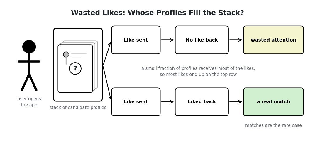
    Line-art scene: a user in front of a phone showing a stack of profile cards with a question mark, one branch where a sent like is ignored and another where it is returned as a match

    The Problem: every card in the stack spends a user’s finite attention, and a like that is never returned buys nothing for either side. The design question is which profiles deserve those thirty slots.

    Answer

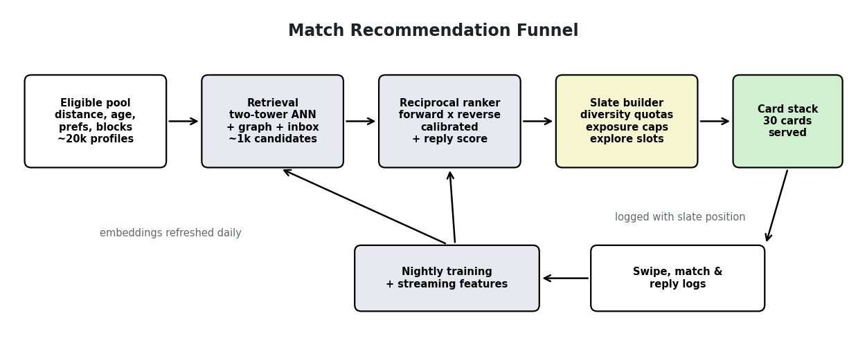
    The design is a four-stage funnel: hard filters cut the global user base to an eligible geo and preference pool, an embedding retrieval stage pulls roughly a thousand candidates, a reciprocal ranker scores each pair by the probability of a mutual like, and a slate builder assembles the actual stack under diversity, exposure, and exploration quotas. Two decisions carry the answer. First, the ranking objective is expected mutual match, p_{uv} \cdot p_{vu}, not one-sided like probability, because a one-sided like is wasted attention on both sides of the market. Second, the system is treated as a two-sided marketplace with a scarce resource (each user’s daily attention and inbox capacity), so popular profiles get exposure caps and under-exposed profiles get guaranteed slots instead of being buried by a pure desirability ranking.
    (1) Hard Filters First: distance, age band, gender preference, blocks, and recent-activity recency are non-negotiable constraints applied before any model, shrinking millions of profiles to tens of thousands.
    (2) Two-Tower Retrieval: geo-sharded ANN lookup over profile embeddings plus complementary sources (mutual-graph, recently-active, likes-you inbox) returns about a thousand candidates in tens of milliseconds.
    (3) Reciprocal Ranker: a shared-encoder model with a forward head and a reverse head predicts both directions and ranks by the calibrated product, so a wildly popular profile who will never swipe back scores below a plausible mutual.
    (4) Exposure Allocation: per-profile impression caps, inbox-load damping, and demand-aware discounting spread likes across the tail instead of concentrating them on the top decile.
    (5) Slate With Explore Slots: the stack is built as a slate, not a top-k list, with quotas for diverse archetypes, uncertain pairs, and new users, which is also how the system escapes the filter bubble.
    (6) Retention-Aligned Objective: the training label mix and slate quotas are tuned against day-7 and day-28 retention and conversation rate, not swipe volume.

    Pipeline diagram: eligible pool after hard filters, two-tower retrieval, reciprocal ranker, slate builder with caps and exploration, served card stack, with swipe logs feeding training back into retrieval and ranking

    Figure 1: The funnel: filters remove the impossible, retrieval proposes, the reciprocal ranker scores both directions, and the slate builder decides what the user actually sees.

    Clarify Before Designing:
    (1) Scale And Density: how many daily active users, and how dense is a typical market (a dense city with 50k eligible profiles behaves nothing like a rural area with 300)?
    (2) Product Grammar: is it a fast swipe stack (Tinder style, roughly 100 cards per session) or a small curated set (Hinge style, a handful per day)? The slate size changes the whole exploration budget.
    (3) Success Definition: is the north star matches, conversations that reach a reply, dates, or subscription retention? Optimizing matches alone rewards low-quality likes.
    (4) Latency And Precompute: can we precompute a stack asynchronously between sessions, or must every card be scored at request time?
    (5) Fairness And Policy Constraints: which attributes may the ranker use, what exposure floor do we owe new or low-activity users, and are paid boosts part of the allocation?
    (6) Cost Asymmetry: which is worse for retention, a session with zero appealing profiles or an inbox the user cannot keep up with?


    Login to view more content