Tag: LLM

DL0203 LLM Bias Detection Mitigation

How do you detect and mitigate bias in LLM outputs, and what pipeline of classifier scoring, threshold calibration, and mitigation strategies can be applied?

Answer

Bias is not a single scalar you can read off a model, so detection begins by fixing a measurement protocol rather than by picking a classifier. The standard construction is a counterfactual prompt set in which only a demographic token changes, several sampled generations per prompt under fixed decoding parameters, and a scorer ensemble that turns each generation into numbers (toxicity, regard, sentiment, stereotype agreement, refusal). The quantity that matters is then a gap between groups with a confidence interval, not an absolute score, because every scorer has an offset that cancels when you subtract. Only after the gaps are measured does thresholding enter, and a single global threshold is almost always wrong because the guard classifier has its own group-dependent error rates. Mitigation is a ladder from cheap and reversible to expensive and durable: system-prompt constraints, decode-time filtering with rewrite, preference tuning on paired data, and finally changes to the pretraining or SFT mixture. The hardest part in production is that the detector and the model must be evaluated together, since a biased guard silently converts fairness work into unequal censorship.

(1) Counterfactual Prompt Design: generate matched pairs where only the group term varies, so any score difference is attributable to that token rather than to topic or length.
(2) Scorer Ensemble, Not One Classifier: a toxicity head, a regard/sentiment head, a rubric-driven LLM judge, and a refusal detector disagree in useful ways; a single classifier both misses stereotype-without-toxicity and over-flags reclaimed language.
(3) Gaps With Uncertainty: report $\Delta_{ab}$ with a bootstrap confidence interval per slice, because a 2-point gap on 40 prompts is noise and a 2-point gap on 4,000 prompts is a launch blocker.
(4) Threshold Calibration Per Slice: choose the operating point from a per-group FPR target on benign text, and record how far apart the group thresholds have to be; that distance is itself a bias metric of the guard.
(5) Mitigation Ladder: system prompt → decode-time filter and rewrite → counterfactual data augmentation and DPO → data-mixture change, in increasing cost, latency impact, and durability.
(6) Guard The Guard: toxicity classifiers show measured dialect bias, so evaluate the detector on group-labelled benign text before you trust any gate it powers.

Left-to-right pipeline: counterfactual prompt pairs feed the LLM under test with eight samples per prompt at fixed decoding, which fans out to three scorers (toxicity and regard classifier, stereotype LLM judge with rubric, refusal and sentiment detector), which feed per-group aggregation of gaps with bootstrap confidence intervals, then a threshold gate calibrated per group at five percent false-flag rate, which routes to allow, rewrite and re-sample, or refuse and log slice; a bottom loop sends aggregated gaps into an offline mitigation box covering counterfactual data augmentation, DPO on paired preferences, activation steering, and a tighter system prompt, which feeds back into the model

Figure 1: The measurement half of the pipeline is online and the mitigation half is offline. The gate on the right acts on a single generation, while the aggregation block is the only place where a bias claim can legitimately be made, because bias lives in a distributional gap and not in any individual score.

Two implementation details decide whether the numbers mean anything. First, decoding must be frozen across the counterfactual arms: temperature, top-p, seed policy, and sample count identical, otherwise you are measuring sampling variance. Second, refusals must be scored separately. A model that answers a question about one group and declines the matched question about another has a large refusal-rate gap while showing a near-zero toxicity gap, and a pipeline that only tracks toxicity will report the model as clean. On the mitigation side, the same discipline applies in reverse: any intervention must be re-measured on the identical prompt set plus a general-capability suite, because prompt-level and decode-time fixes routinely buy a lower gap at the price of higher refusal on benign requests, which is a regression that no bias dashboard shows.

Mathematical Formulation:
$s = f_{\phi}(x, y) \in [0, 1]$
$\Delta_{ab} = \mathbb{E}[s \mid g = a] - \mathbb{E}[s \mid g = b]$
$\mathrm{FPR}_g(\tau) = P(s > \tau \mid g, \mathrm{benign})$
$\tau_g = \min \{ \tau : \mathrm{FPR}_g(\tau) \leq \alpha \}$
$\mathrm{ECE} = \sum_{b=1}^{B} \frac{n_b}{N} |\bar{s}_b - \bar{y}_b|$

Where:

$s$ is the scorer output for prompt $x$ and generation $y$ , produced by a guard classifier or judge with parameters $\phi$ that are separate from the model under test.
$g$ is the group or slice label attached to the prompt (demographic term, dialect, language), and $a, b$ are the two arms of a counterfactual pair.
$\Delta_{ab}$ is the group gap, the primary detection statistic; it is reported with a bootstrap interval over prompts, not over samples, since samples within a prompt are correlated.
$\tau$ is the gate threshold and $\alpha$ the tolerated false-flag rate on benign text, so $\tau_g$ is the smallest threshold meeting that budget within group $g$ .
$b \in \{1, \ldots, B\}$ indexes confidence bins with $n_b$ items out of $N$ ; $\bar{s}_b$ is the mean score and $\bar{y}_b$ the empirical label rate, so ECE measures whether a score of 0.7 actually means 70% harmful.

Worked Calibration Example (5,000 benign sentences per group):
$\mathrm{FPR}_a(0.50) = 115 / 5000 = 0.023$
$\mathrm{FPR}_b(0.50) = 455 / 5000 = 0.091$
$\tau_a = 0.40$
$\tau_b = 0.58$

The same threshold of 0.50 therefore flags benign text from group $b$ roughly four times as often, and equalizing the false-flag rate at $\alpha = 0.05$ requires thresholds 0.18 apart. That spread is the diagnostic: it says the guard classifier, not the generator, is the largest bias source in the stack, and the correct response is usually to fix the classifier’s training data rather than to ship group-conditional thresholds.

Line chart of false-flag rate on benign text versus gate threshold for two groups, both decreasing curves with group B consistently above group A; a vertical dashed line at threshold 0.5 meets the curves at 2.3 percent and 9.1 percent, a horizontal line marks the 5 percent target, and two circular markers show the per-group thresholds 0.40 and 0.58 that achieve 5 percent each

Figure 2: A single operating point produces two different error rates. Reading the gate at fixed threshold hides the disparity, while reading it at fixed false-flag rate exposes it as a horizontal distance between the two curves, which is the quantity to drive toward zero when you retrain the guard.

Property	Prompt / system level	Decode-time filter and rewrite	Training-time (CDA, DPO)
Where it acts	Instruction and few-shot context, no weight change	Guard score on the sampled output, then re-sample or refuse	Weights, via augmented pairs or preference optimization
Cost to ship	Hours, revertible with a config push	One extra forward pass per output, plus rewrite latency on flags	Days of data work and a full eval cycle per iteration
Durability	Low, defeated by paraphrase and long context drift	Medium, bounded by the guard’s own recall and calibration	High, the behaviour itself moves rather than being masked
Dominant failure mode	Over-refusal on benign group-related questions	Inherits the classifier’s dialect bias, so filtering is unequal	Capability regression and reward hacking of the preference signal
What to measure after	Refusal-rate gap on benign prompts per slice	Per-group FPR at fixed threshold, plus added p95 latency	Counterfactual gap, general benchmarks, and win rate versus baseline

August 21, 2026

DL0201 Pretraining Loss Spike Debugging

During pretraining of a 100B parameter model on a large GPU cluster, you suddenly see loss spikes. How do you debug this, and is it a data issue, a learning-rate problem, or hardware failure?

Answer

All three causes are real at this scale, and they leave different fingerprints, so the answer is a triage order rather than a guess. Run the checks in order of cost: first the numerics and per-rank logs you already have on disk (NaN or Inf, one data-parallel rank far from the mean loss, XID or ECC events, NCCL timeouts), then the optimizer traces (global gradient norm, Adam update ratio, maximum attention logit, output logit magnitude), and only then the data, which is proven guilty only by replaying the exact batch from the pre-spike checkpoint. The shape of the curve already narrows the space: a single sharp spike that recovers within a few thousand steps is usually a batch-times-model-state interaction, a slow creeping divergence preceded by growing logits is a learning-rate or numerics problem, and an instant jump to NaN with a stalled step time is hardware. The industry-standard mitigation for the first case is the one PaLM reported: rewind to a checkpoint roughly 100 to 200 steps before the spike and skip a few hundred batches, which removes the spike even though the same data is harmless from a different model state. That asymmetry is the single most important fact in this debugging problem, because it means “the data was bad” is almost never the correct conclusion on its own.

(1) Read The Shape First: recoverable spike, creeping divergence, and hard fault are three distinct signatures, and each maps to a different subsystem.
(2) Cheapest Check First: numerics and per-rank divergence cost nothing to inspect, optimizer traces cost one dashboard query, and a batch replay costs about one node-hour.
(3) Never Trust The Global Loss: with 512 data-parallel ranks a single sick rank moves the average by a fraction of a percent, so log per-rank loss and gradient-norm maxima, not just the mean.
(4) Silent Data Corruption Has No NaN: a degrading GPU can return wrong arithmetic with no error flag, so keep a bitwise-reproducibility canary that reruns one batch on two hosts and compares.
(5) Data Is Guilty Only On Replay: rerun batch $b_s$ from the checkpoint at step $s-1$ on a fresh replica; if the spike does not reproduce, the batch is not the cause.
(6) Skip-And-Resume Versus Config Change: rollback is right for isolated spikes, but recurring spikes plus growing attention logits mean you must pay for QK-norm, z-loss, a lower peak learning rate, or fp32 optimizer state.

Two-row by three-column chart grid. Top row shows training loss versus step for three cases: a single sharp spike at step 9000 that recovers to trend, a creeping divergence starting near step 11500 that never returns, and a curve that ends abruptly at step 15000 with a NaN marker. Bottom row shows the corresponding global gradient norm on a log scale with a clipping threshold line at 1.0: a single narrow 15x spike, a gradient norm that creeps up for two thousand steps before the loss moves, and a flat trace that terminates in an infinite value.

Figure 1: The same symptom, three diseases. Case A is a recoverable spike whose gradient norm spikes for a handful of steps and then returns, case B is a creeping divergence in which the gradient norm rises for roughly 2,000 steps before the loss visibly moves, and case C is a hard fault with no precursor at all. Note that gradient clipping at 1.0 caps the applied update but does not hide the raw norm, which is exactly why the raw norm must be logged.

The mechanism behind case B is worth being precise about, because it is the one people misdiagnose as bad data. As training proceeds, attention logits $q_i^\top k_j / \sqrt{d_h}$ can grow without bound; the softmax saturates, one head collapses onto a single position, and the gradient through that head becomes both tiny and extremely sharp. In parallel, the output logits drift so that $\log Z$ wanders, which makes the cross-entropy surface stiff in a direction the optimizer cannot see from the loss value alone. Case A has a different mechanism: in bf16 or when optimizer state is stored in low precision, the Adam second moment for a rarely-activated parameter block (embeddings for rare tokens are the classic example) can decay toward the epsilon floor, after which one moderate gradient produces an update whose effective step size is orders of magnitude larger than intended. The debugging pipeline is therefore always the same: detect → localize → replay → mitigate, with instrumentation decided before the run rather than after the first spike.

Mathematical Formulation:
$\ell_t > \mu_{t-W:t} + 3\,\sigma_{t-W:t}$
$\theta_{t+1} = \theta_t - \eta_t \dfrac{\hat m_t}{\sqrt{\hat v_t} + \epsilon}$
$r_t = \dfrac{|\hat m_t|}{\sqrt{\hat v_t} + \epsilon}$
$r_{\max} \approx \dfrac{1-\beta_1}{\sqrt{1-\beta_2}}$
$s_{ij} = q_i^\top k_j / \sqrt{d_h}$
$\mathcal{L} = \mathcal{L}_{\mathrm{CE}} + \alpha (\log Z)^2$

Where:

$\ell_t$ is the training loss at step $t$ , and $\mu$ and $\sigma$ are the mean and standard deviation over a trailing window of $W$ steps (a few hundred works well); this is the spike detector that should fire an alert, not a human eye on a dashboard.
$\theta_t$ are the parameters, $\eta_t$ the scheduled learning rate, and $\hat m_t$ and $\hat v_t$ the bias-corrected first and second Adam moments with decays $\beta_1$ and $\beta_2$ .
$r_t$ is the update ratio, the per-block quantity to log alongside the gradient norm, because it exposes the actual step size the optimizer is taking rather than the size of the gradient.
$r_{\max}$ is the ratio a single outlier gradient can produce, roughly $0.1/\sqrt{0.05} \approx 0.45$ for $\beta_1 = 0.9$ and $\beta_2 = 0.95$ ; this bound holds only while $\sqrt{\hat v_t}$ dominates $\epsilon$ , and it is epsilon underflow that breaks it.
$s_{ij}$ is the pre-softmax attention logit for query $i$ and key $j$ with head dimension $d_h$ ; tracking $\max_{ij} |s_{ij}|$ per layer is the earliest available warning of the creeping-divergence mode.
$Z = \sum_{v=1}^{V} \exp(z_v)$ is the softmax partition function over vocabulary size $V$ , and $\alpha$ is the z-loss coefficient (commonly $10^{-4}$ ) that pins $\log Z$ near zero at negligible quality cost.

The $r_{\max} \approx 0.45$ bound is the reason “one weird document blew up the run” is usually wrong: with healthy second moments, Adam already damps a single 30x outlier gradient to less than a normal step. What actually hurts is a sequence of correlated large gradients, or a block whose $\hat v_t$ has collapsed so that the denominator is dominated by $\epsilon$ . That distinction determines the fix: correlated gradients are a data-ordering and learning-rate problem, while a collapsed second moment is a precision problem solved by keeping optimizer state in fp32 and raising $\epsilon$ .

Left-to-right triage diagram. A trigger box for a detected loss spike fans out to three ordered check boxes: numerics and per-rank divergence, optimizer signals such as gradient norm and maximum attention logit, and a replay of the offending batch from the previous checkpoint. Each check has a yes branch to an evidence box listing concrete symptoms, and each evidence box points to a verdict box: hardware, learning rate and numerics, or data crossed with model state. Vertical clean arrows connect check one to check two and check two to check three.

Figure 2: The triage order that makes this question answerable in an interview. The three branches are ordered by cost per bit of information, not by likelihood, and the replay step is what separates a genuinely corrupt shard from a batch-times-state interaction that a 400-batch skip will silently fix.

Signal	Data and model state	Learning rate and numerics	Hardware and interconnect
Loss shape	Sharp isolated spike, recovers to trend within a few thousand steps	Repeated spikes of growing size, or a divergence that never recovers	Instant NaN or Inf, or a flat line while step time stalls
Gradient norm	One narrow burst of a few steps, clipping engages briefly	Slow upward drift over thousands of steps, clipping engages permanently	Jumps straight to Inf, or becomes exactly zero on one rank
Per-rank pattern	Elevated on the ranks holding the offending microbatches only	Uniform across all ranks, since the cause is the shared update	One rank or one host is an extreme outlier, or a canary mismatches bitwise
Replay test	Reproduces from the same checkpoint, disappears from a different one	Reproduces from any nearby checkpoint with the same schedule	Does not reproduce on a healthy node with identical inputs
Corroborating logs	Sample dump shows repeated n-grams, a truncated shard, or non-text bytes	Max attention logit and update ratio rising, parameter norm inflating	XID or ECC entries, NCCL timeouts, thermal throttling, link flaps
First mitigation	Rewind about 200 steps, skip 200 to 500 batches, then dedup or drop the shard	Lower peak LR, extend warmup, add QK-norm and z-loss, keep fp32 optimizer state	Fence the host, restore the last checkpoint, rerun on a spare node

The operational context matters for how much of this you should automate. Meta reported 419 unexpected interruptions during Llama 3 405B pretraining, with roughly 78% traced to hardware, which means at 100B scale a fault-driven anomaly is not an exotic event but a weekly one. That argues for treating spike response as a control loop: an automatic detector on the trailing-window rule, automatic checkpoint retention dense enough to rewind 200 steps, automatic host fencing on XID events, and a human decision only for the residual class where the numerics themselves are unstable.

August 21, 2026

DL0199 Sensitive Data Memorization Remediation

Imagine you’ve trained a model with unusually strong memorization of sensitive data. What steps would you take next?

Answer

Handle it as a privacy incident with a measurement problem at its core, not as a modeling curiosity. The first hour is containment: stop the rollout, pin and lock every checkpoint derived from the suspect run, and bring legal and privacy owners in immediately, because notification clocks (for example the 72-hour clock in GDPR Article 33) start from awareness rather than from confirmation. Then quantify before you touch anything, since “the model memorizes” is not an actionable statement until you have a per-record extraction rate under an adversarial prompt distribution, a canary exposure number, and a membership-inference AUC. Diagnosis almost always lands on the same few causes: near-duplicate records, personal data that survived scrubbing because it arrived through production logs, or too many epochs over a small sensitive shard. Only then do you pick the cheapest remediation tier that clears an agreed risk gate, escalating output guard → targeted unlearning → retrain with deduplication and DP-SGD, and you verify with adversaries you did not design the fix against.

(1) Contain Before You Explain: Freeze the rollout, revoke external checkpoint and API access, and preserve prompts, completions, and data manifests so the incident can be scoped later.
(2) Quantify With Adversarial Probes: Report extraction rate under prefix, divergence, and template attacks plus canary exposure in bits, not a handful of prompts that happened to leak.
(3) Duplication Is The Usual Root Cause: A record repeated a dozen times is far more extractable than a record seen once, so a near-duplicate audit on the flagged records comes before any algorithmic fix.
(4) Use A Cost-Ordered Remediation Ladder: Output filters buy hours, targeted unlearning buys weeks, and only retraining with deduplication and DP-SGD yields a formal per-record bound.
(5) Verification Must Be Independent: Re-measure on held-out canaries and an adaptive red team, check utility regressions, and probe for relearning, because suppressed knowledge often returns after light fine-tuning.
(6) Deletion Obligations Propagate: Embeddings, indexes, eval logs, distilled students, and downstream fine-tunes all inherit the memorization, so the remediation plan must enumerate every derived artifact.

Serpentine incident-response flow: top row contains contain, quantify and diagnose stages; the middle row is an escalating remediation ladder read right to left from output guard to targeted unlearning to full retrain with deduplication and differential privacy, with escalate arrows between tiers; the bottom row runs verify, monitor and close out

Figure 1: The playbook, ordered by cost rather than by ambition. Each escalation step is triggered by a failed risk gate, not by preference, and the loop only closes when independent probes and a documented data lineage both hold.

The measurement phase decides everything downstream, so it deserves real engineering. Insert canaries (synthetic secrets with known formats and known insertion counts) into future runs, and for the current model estimate exposure by ranking the true secret against a candidate set of same-format alternatives under the model’s own likelihood. Complement this with black-box extraction rate: run a large, adversarially generated prompt set and count verbatim recoveries of records you know are in the training set. Two subtleties trip teams up. A single leaked record is enough to be reportable, so the metric that matters is a confidence bound on the leak probability rather than a point estimate. And zero observed hits is not zero risk: with no hits in $N$ probes, the 95% upper bound on the per-probe rate is about $3/N$ , which is why a 200-prompt smoke test can never clear a production gate.

Mathematical Formulation:
$\mathrm{exposure}(s) = \log_2 |\mathcal{R}| - \log_2 \mathrm{rank}(s)$
$\mathrm{rank}(s) = |\{ r \in \mathcal{R} : \mathcal{P}(r) \leq \mathcal{P}(s) \}|$
$\hat{e} = \frac{1}{N} \sum_{i=1}^{N} \mathbf{1}[ g(p_i) = s_i ]$
$\hat{e} = 0 \Rightarrow p_{95} \approx 3/N$
$\Pr[M(D) \in S] \leq e^{\epsilon} \Pr[M(D') \in S] + \delta$

Where:

$s$ is the sensitive string under test and $\mathcal{R}$ the set of same-format candidates it is ranked against, so $\log_2 |\mathcal{R}|$ (30 bits for a 9-digit-scale secret) is the maximum exposure.
$\mathcal{P}(\cdot)$ is the model’s perplexity of a candidate; $\mathrm{rank}(s) = 1$ means the true secret is the model’s single most likely completion.
$\hat{e}$ is the empirical extraction rate, $p_i$ the $i$ -th adversarial prompt, $g$ the decoding procedure, and $N$ the number of probes.
$p_{95}$ is the 95% upper confidence bound on the per-probe leak probability, which is the number a risk gate should be written against.
$M$ is the training mechanism, $D$ and $D'$ two datasets differing in one record, and $(\epsilon, \delta)$ the differential privacy budget that bounds any single record’s influence on the released weights.

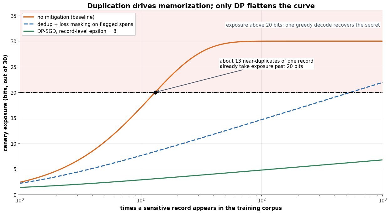
Log-scale chart of canary exposure in bits against the number of times a sensitive record appears in the training corpus, showing a baseline curve that saturates near 30 bits after a few dozen duplicates, a slower curve for deduplication plus loss masking, and a nearly flat curve for DP-SGD training, with a shaded region above 20 bits marking where a single greedy decode recovers the secret

Figure 2: Why the duplicate audit comes first. Under ordinary training, roughly 13 near-duplicates of one record are enough to push exposure past 20 bits, where a single greedy decode recovers it; mitigations such as span masking only shift the curve right, while DP-SGD flattens it at the cost of long-tail accuracy.

Remediation tier	3a. Output-side guard	3b. Targeted unlearning	3c. Retrain (dedup + DP-SGD)
What it changes	Decoding and post-processing only; weights untouched	Weights, via a forget-set objective on the flagged records	The data pipeline and the training objective, from a clean checkpoint
Time to deploy	Hours	Hours to days	Days to weeks
Compute cost	Negligible, plus per-token filter latency	Roughly 0.1 to 1 percent of the original training FLOPs	A full training budget, plus DP-SGD clipping overhead
Guarantee	None; only block-list coverage of known strings	Empirical and benchmark-dependent; reversible by relearning	Formal per-record bound with a stated epsilon and delta
Utility cost	Near zero, aside from false blocks on common strings	Measurable drift on neighboring, legitimate knowledge	Largest on rare classes and long-tail facts
Dominant failure mode	Paraphrase, translation, or encoding walks around the match	The fact is still latent; only the surface form is suppressed	Epsilon accounting is void if one record recurs under many users

August 21, 2026

DL0198 TF-IDF Vectorization

What is TF-IDF vectorization, how does it combine term frequency and inverse document frequency to weight words, and what are its limitations compared to embedding-based representations?

Answer

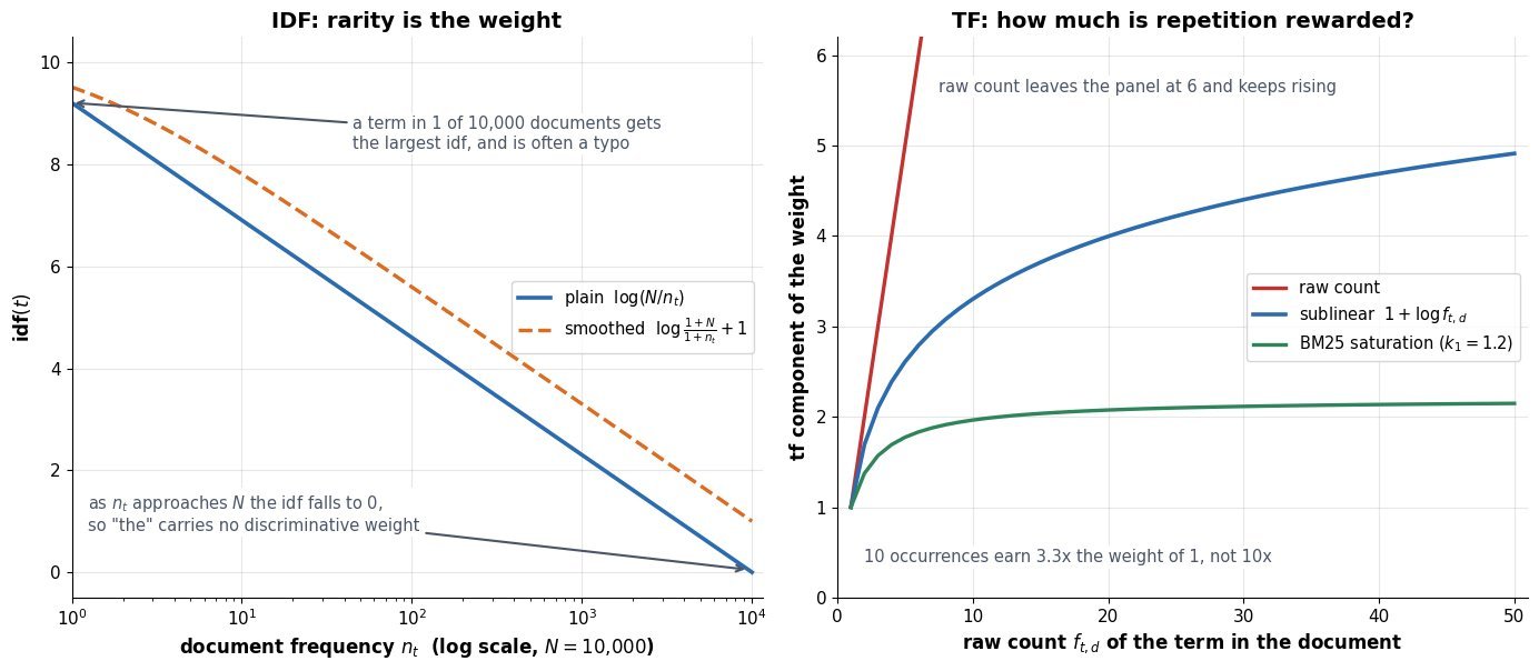
TF-IDF maps each document to a vector whose length equals the vocabulary size, where coordinate $t$ holds a weight that rises with how often term $t$ occurs in that document and falls with how many documents in the corpus contain it. The term-frequency factor is local and per-document, usually damped as $1 + \log f_{t,d}$ so that ten occurrences do not count ten times as much as one. The inverse document frequency factor is a global corpus statistic, $\log(N/n_t)$ , which pushes function words such as “the” toward zero and lifts rare, discriminative terms. Multiplying the two produces the classic “frequent here, rare elsewhere” signal, and L2 normalization turns a plain dot product into cosine similarity. The result is extremely sparse (typically over 99.9% zeros), exactly interpretable per term, and requires no training beyond counting. Its weaknesses are structural rather than fixable by tuning, because every term is its own orthogonal dimension, so “car” and “automobile” share zero similarity, word order and negation are discarded, and any term outside the fitted vocabulary is silently dropped.

(1) Two Factors, Two Scopes: tf is computed from one document, idf from the whole corpus, and the product is what makes a term both present and distinctive.
(2) Sublinear Damping: raw counts overweight repetition, so $1+\log f_{t,d}$ or BM25 saturation caps the reward for saying the same word again.
(3) IDF Is Fitted, Not Computed Per Query: the $n_t$ statistics are frozen at fit time, so corpus drift, duplicated documents, and tiny corpora all distort the weights.
(4) Normalization Removes Length Bias: without L2 (or pivoted) normalization long documents dominate every ranking simply by containing more words.
(5) Sparse Means Cheap And Exact: an inverted index serves lexical matches on CPU in milliseconds, and high idf makes SKUs, error codes, and legal citations very precise.
(6) The Structural Limits: orthogonal vocabulary dimensions mean no synonymy or paraphrase, bag-of-words means no order or negation, and out-of-vocabulary terms contribute nothing at all.

Mathematical Formulation:
$w_{t,d} = \mathrm{tf}(t,d)\cdot \mathrm{idf}(t)$
$\mathrm{tf}(t,d) = 1 + \log f_{t,d}$
$\mathrm{idf}(t) = \log \frac{N}{n_t}$
$\mathrm{idf}_{s}(t) = \log \frac{1+N}{1+n_t} + 1$
$\hat{w}_{d} = w_{d} / \|w_{d}\|_2$
$\mathrm{sim}(q,d) = \hat{w}_{q}^{\top}\hat{w}_{d}$

Where:

$w_{t,d}$ is the unnormalized weight of term $t$ in document $d$ , and $\hat{w}_{d}$ is the final L2-normalized document vector.
$f_{t,d}$ is the raw count of $t$ in $d$ , defined only for $f_{t,d} \geq 1$ ; terms with zero count keep weight zero, which is what makes the vector sparse.
$N$ is the number of documents in the fitted corpus and $n_t$ the document frequency, the number of documents containing $t$ , so $1 \leq n_t \leq N$ .
$\mathrm{idf}_{s}$ is the smoothed variant used by scikit-learn, which adds one to both counts to tolerate unseen terms and adds a constant so a term present everywhere still keeps a small nonzero weight.
$q$ is the query treated as a short pseudo-document, so retrieval scoring is just a cosine between two sparse vectors over shared nonzero coordinates.

Worked IDF Example (natural log, one million documents):
$\mathrm{idf}(\mathrm{the}) = \log(10^6/10^6) = 0$
$\mathrm{idf}(\mathrm{car}) = \log(10^6/10^5) = 2.30$
$\mathrm{idf}(\mathrm{sarcoidosis}) = \log(10^6/50) = 9.90$

The spread of those three numbers is the whole mechanism. A stopword is annihilated without any hand-written stoplist, a common content word keeps a moderate weight, and a domain-specific term is worth roughly four common words in the same document. That also exposes the fragility: a term appearing in exactly one document receives the maximum weight even when it is a typo, an OCR error, or a hash, which is why production pipelines cap the vocabulary with min_df and max_df thresholds instead of trusting idf alone.

Two panels: on the left, inverse document frequency plotted against document frequency on a log x-axis for a corpus of ten thousand documents, comparing the plain log of N over n_t against the smoothed scikit-learn variant, with annotations at the rare-term and stopword ends; on the right, three term-frequency transforms plotted against raw term count, showing the raw linear count leaving the panel, the sublinear one-plus-log curve, and BM25 saturation flattening near two point two

Figure 1: The two factors behave very differently. IDF decays logarithmically in document frequency and reaches zero for a term present in every document, while the tf transform decides how much repetition is rewarded: raw counts grow without bound, $1+\log f_{t,d}$ gives a tenfold count only 3.3 times the weight of a single occurrence, and BM25 saturation is asymptotically bounded by $k_1+1$ .

BM25 is the natural upgrade inside the sparse family, replacing the log-tf term with an explicitly saturating form plus document-length normalization, and it usually beats plain TF-IDF on ranking while keeping the same inverted index. What neither can do is bridge vocabulary mismatch. In a TF-IDF space the coordinates for “car”, “automobile”, and “voiture” are mutually orthogonal, so a query using one word scores exactly zero against a document using another, no matter how many synonyms both share in meaning. Embedding-based representations solve this by construction, mapping text into a dense $\mathbb{R}^{d}$ with $d$ typically between 384 and 1024, where distributional training places related words and paraphrases close together and sub-word tokenization guarantees that nothing is out of vocabulary. The price is real: an encoder needs pretraining plus contrastive fine-tuning, similarity becomes uninterpretable, and dense retrievers can drift badly out of domain, which is exactly where exact lexical matching on an identifier still wins.

Left panel shows a six-term by five-document TF-IDF matrix as a grayscale heatmap with numeric cell values, where the row for the stopword the is all zeros and the rows for car and automobile never share a nonzero column; right panel sketches a dense embedding space as unit arrows from the origin, with car, automobile, and vehicle pointing in nearly the same direction, insurance rotated away, and banana pointing into a different quadrant

Figure 2: Left, a TF-IDF matrix is mostly zeros and each term owns its own axis, so the “car” and “automobile” rows never overlap and their cosine similarity is exactly 0. Right, a dense encoder places the same synonyms at a small angle, which is what recovers paraphrase recall while giving up the per-term readability of the sparse weights.

Property	TF-IDF / BM25 (sparse lexical)	Dense embeddings (bi-encoder)
Dimensionality	Vocabulary size, 50k to 1M, over 99.9% zeros per document	Fixed 384 to 1024 dense floats, fully populated
Fitting cost	One counting pass, no gradients, minutes on CPU	Pretraining plus contrastive fine-tuning on paired data
Synonyms and paraphrase	None: distinct surface forms are orthogonal dimensions	Captured: near-duplicate meanings land at small angles
Rare exact strings	Strong: high idf makes SKUs and error codes highly selective	Weak: rare identifiers are blurred into nearby token directions
Unseen terms	Dropped silently at transform time, contributing nothing	Always representable through sub-word tokenization
Order and negation	Lost, unless n-grams are added at a cost in dimensionality	Partly encoded by the contextual attention layers
Serving	Inverted index, CPU, millisecond lookups, trivial updates	ANN index such as HNSW or IVF, GPU for encoding queries
Dominant failure mode	Vocabulary mismatch gives zero recall on paraphrased queries	Out-of-domain drift returns topically close but wrong documents

August 21, 2026

DL0196 Reward Model Overfitting

How do you prevent the reward model from overfitting in RLHF, and what role do data diversity, ensemble reward models, and uncertainty estimation play?

Answer

A reward model (RM) is a learned proxy for human judgement fitted on a finite set of preference pairs, so it fails in two distinct ways that need different defenses. The first is ordinary statistical overfitting: held-out pairwise accuracy typically plateaus in the 65-75% band and then degrades, which is why InstructGPT-era practice is a single epoch at a small learning rate, since a second epoch mostly memorizes annotator noise. The second and more damaging failure is over-optimization, where held-out accuracy still looks acceptable but the policy drifts into a region the RM never saw labeled, so the proxy score climbs while true human preference falls. The defenses are therefore spread across the whole loop rather than concentrated in the RM training script. Diverse prompts and on-policy responses widen the region where the RM is actually supervised, an ensemble of independently seeded RMs converts the unsupervised region into a measurable disagreement signal, and a pessimistic aggregate such as mean minus $\lambda$ times the spread turns that signal into a reward the policy cannot profit from. A KL penalty to the frozen reference policy plus periodic relabeling of fresh on-policy samples keeps the optimizer inside the RM’s zone of competence.

(1) Two Different Failures: Classical overfitting is measured on held-out preference pairs, while over-optimization is a Goodhart effect visible only when the RM is used as an RL objective. Fixing one does not fix the other.
(2) Train Short, Regularize Hard: One epoch, learning rates around $10^{-5}$ or below, early stopping on held-out pairwise accuracy, plus label smoothing or a margin term and an auxiliary language-modeling loss to keep the backbone from collapsing.
(3) Data Diversity Sets The Support: Prompts from real traffic, red-teaming, and synthetic edge cases, with responses sampled from several policy checkpoints and temperatures, so the RM is supervised where the policy will actually go.
(4) Multiple Annotators Bound The Ceiling: Human agreement of roughly 70-80% on subtle pairs caps achievable accuracy, so a model chasing 90% training accuracy is fitting noise, not preference.
(5) Ensembles Estimate Epistemic Uncertainty: $K = 3$ to $5$ members whose pretraining seeds differ disagree most off-distribution, which is exactly where reward hacking begins.
(6) Pessimism Turns Uncertainty Into Reward: Optimizing a lower confidence bound or the worst-of- $K$ score delays the over-optimization peak instead of merely detecting it.
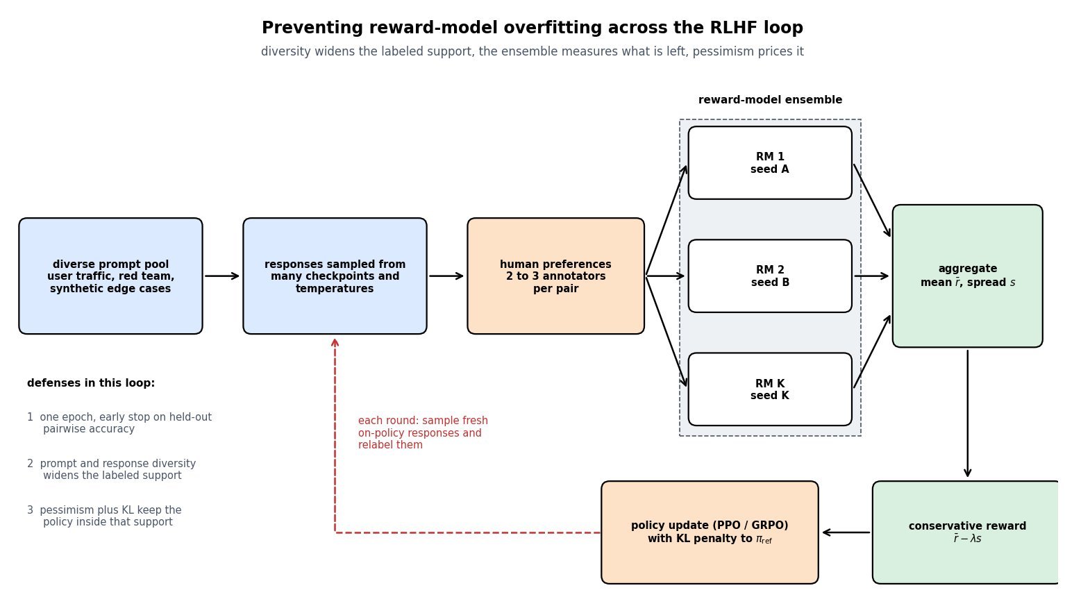
(7) Close The Loop: Iterative rounds that relabel on-policy samples attack the root cause, distribution shift, rather than its symptom.

Loop diagram: a diverse prompt pool feeds response sampling from many policy checkpoints and temperatures, which feeds human preference labeling with two to three annotators per pair, which trains an ensemble of K reward models with independent pretrain seeds, whose outputs are aggregated into a mean and a spread, converted into a conservative reward equal to the mean minus lambda times the spread, and used by a PPO or GRPO policy update with a KL penalty, with a dashed feedback edge sending fresh on-policy responses back for relabeling each round

Figure 1: Where each defense sits in the loop. Diversity widens the labeled support, $K$ independently seeded reward models turn unlabeled regions into a measurable spread $s$ , and the conservative reward makes the policy pay for that spread. The dashed feedback edge is the only mechanism that actually removes distribution shift rather than penalizing it.

Data diversity is the highest-leverage lever because it changes the support of the training distribution rather than the fit on a fixed support. Preference sets collected from one prompt source and one policy checkpoint produce an RM that is accurate on that slice and arbitrary elsewhere, and the policy will find “elsewhere” within a few thousand PPO steps. Two diversity axes matter most: the prompt distribution, which should mix production traffic, adversarial red-team prompts, and long-tail synthetic cases, and the response distribution, which should include samples from several checkpoints, several temperatures, and deliberately balanced lengths so the RM does not learn that longer equals better. Multi-annotator labeling on a subset gives the agreement rate, and that rate is the practical accuracy ceiling: driving training accuracy far past it is a direct measurement of memorization.

Mathematical Formulation:
$\Delta_\theta = r_\theta(x, y_w) - r_\theta(x, y_l)$
$\mathcal{L}_{\mathrm{RM}} = -\log \sigma(\Delta_\theta)$
$\bar r(x,y) = \frac{1}{K}\sum_{k=1}^{K} r_k(x,y)$
$s^2(x,y) = \frac{1}{K}\sum_{k=1}^{K}(r_k - \bar r)^2$
$r_{\mathrm{LCB}} = \bar r - \lambda s$
$J(\pi) = \mathbb{E}_{\pi}[r_{\mathrm{LCB}}] - \beta D_{\mathrm{KL}}$

Where:

$\Delta_\theta$ is the score margin between the preferred response $y_w$ and the rejected response $y_l$ for prompt $x$ , and $\sigma$ is the logistic function, so $\mathcal{L}_{\mathrm{RM}}$ is the Bradley-Terry negative log-likelihood.
$\theta$ are the RM parameters: a pretrained or SFT backbone with a scalar head, usually trained for one epoch so $\mathcal{L}_{\mathrm{RM}}$ never approaches zero.
$r_k$ is the score of ensemble member $k \in \{1,\ldots,K\}$ , and $\bar r$ their mean, which is also a mild variance reduction on the reward itself.
$s(x,y)$ is the ensemble spread, used as an epistemic uncertainty proxy: it stays small on the labeled support and grows on responses no annotator ever judged.
$\lambda \geq 0$ is the pessimism coefficient, commonly in the range $0.5$ to $2$ ; $\lambda = 0$ recovers plain mean aggregation.
$\beta$ is the KL coefficient (typically $0.01$ to $0.05$ ) and $D_{\mathrm{KL}} = D_{\mathrm{KL}}(\pi \,\|\, \pi_{\mathrm{ref}})$ the divergence from the frozen reference policy, which bounds how far the policy may travel from the RM’s support.

Two-panel chart. Left panel: reward model training accuracy on preference pairs climbing from 0.69 toward 0.98 over four epochs while held-out validation accuracy peaks near 0.73 at one epoch and then declines, with an early-stopping marker at one epoch. Right panel: as policy drift measured by the square root of KL increases, the proxy reward from the reward model rises monotonically, the gold human reward peaks around square root KL of nine and then falls, and a conservative lower-confidence-bound reward reaches a later and higher peak around thirteen

Figure 2: Left: held-out pairwise accuracy peaks near one epoch while training accuracy keeps climbing, which is why single-epoch training with early stopping is the default. Right: the same RM used as an RL objective. The proxy score rises monotonically while the gold reward peaks and then declines, and pessimistic aggregation pushes that peak further out. Curves are schematic and follow the functional form fitted by Gao et al.

The right panel is the empirically important one, and its shape is well described by the over-optimization scaling law, where the gold reward is a function of the drift $d = \sqrt{D_{\mathrm{KL}}}$ rather than of training steps.

Over-Optimization Law:
$R_{\mathrm{gold}}(d) = d\,(a - b \log d)$
$d = \sqrt{D_{\mathrm{KL}}(\pi \,\|\, \pi_{\mathrm{ref}})}$

Here $a$ and $b$ are fitted constants that improve with RM size and with the amount of preference data, so a larger RM trained on more diverse comparisons does not merely score better, it peaks later. Ensembling contributes on two fronts. Averaging $K$ members reduces variance in the reward itself, which stabilizes advantage estimates, and the spread $s$ provides the only cheap in-loop signal that the policy has left the supervised region. In practice the disagreement metric is worth logging even if you never subtract it: a sudden rise in mean $s$ over sampled rollouts is an early warning that arrives before the gold reward turns over. Subtracting it, as in conservative or worst-of- $K$ optimization, costs a little early progress because uncertain but genuinely good responses are also penalized, and buys a substantially later peak. The critical implementation detail is that members must be diverse in their errors: fine-tuning five heads from one pretrained checkpoint with different shuffles yields correlated mistakes, so the spread underestimates true uncertainty precisely on hacked outputs.

Property	Data diversity and relabeling	Ensemble of K reward models	Pessimistic aggregation
What it fixes	Removes the unsupervised region the policy would exploit	Measures that region and reduces reward variance	Makes exploiting that region unprofitable
Mechanism	Widens the support: prompt sources, checkpoints, temperatures, fresh on-policy labels	Spread across members as an epistemic uncertainty proxy	Optimize a lower confidence bound or the worst-of-K score
Typical setting	Relabel every RLHF round; 2 to 3 annotators on a calibration subset	K = 3 to 5, independent pretrain seeds plus bootstrapped data	Pessimism coefficient roughly 0.5 to 2, tuned on gold evaluations
Cost	Human annotation budget and pipeline latency per round	K times training and K times reward-inference compute	Slower early progress; uncertain-but-good responses are penalized
Fails when	Annotators share a bias, such as preferring length or confident tone	Members share a pretrained backbone, so errors correlate	Spread is miscalibrated, so the penalty blocks progress or misses hacks

August 21, 2026

DL0176 Online vs Offline DPO

How does Online DPO, which samples new responses from the current policy during training, differ from Offline DPO on a fixed preference dataset, and why does the online variant generalize better to out-of-distribution prompts?

Answer

Both variants minimize the same Bradley-Terry log-loss over the implicit reward $\hat{r}_\theta = \beta \log (\pi_\theta / \pi_{\mathrm{ref}})$ , so the difference is not the objective but the distribution the training pairs are drawn from. Offline DPO consumes a dataset collected once from some behavior policy, which makes it a purely supervised procedure: four log-probability forward passes per pair, no decoding, and reference log-probs that can be cached before training starts. Online DPO decodes two fresh completions from the current policy at every step, has them ranked by a preference oracle (reward model, LLM judge, or human), and applies the DPO gradient to that on-policy pair, so the data distribution moves as the model moves. The generalization gap follows directly from this. DPO’s derivation only pins the implicit reward down where the data has support, and a frozen dataset’s support stops moving while the policy keeps drifting, so on unfamiliar prompts the model is being shaped by an extrapolated reward that no label ever corrected. On-policy sampling forces the coverage mismatch back toward 1 by construction, so the KL-regularized objective is enforced exactly at the responses the model will actually emit.

(1) Same Loss, Different Sampler: the gradient formula is identical, but offline draws $(y_w, y_l)$ from a fixed $\mu$ while online draws them from $\pi_\theta$ and labels them on the fly.
(2) An Oracle Becomes Mandatory: online DPO needs a ranker in the loop, so the quality ceiling shifts from the dataset to the reward model or judge.
(3) Coverage Versus Exploration: offline guarantees scale with a concentrability coefficient over the whole response space, while on-policy data only needs local coverage around the current policy.
(4) Off-Policy Drift Is Cumulative: every gradient step moves $\pi_\theta$ further from $\mu$ , so the last epoch of offline training is the most off-policy and the least trustworthy.
(5) Cost Is Decode-Bound: an online step adds two autoregressive generations plus an oracle call, typically 5x to 10x the wall-clock of an offline step at the same batch size.
(6) Hybrids Dominate In Practice: iterative or batched online DPO regenerates the preference set every few thousand steps, recovering most of the on-policy benefit at a fraction of the sampling overhead.

Mechanically, offline DPO is a four-forward-pass classification problem. You score the chosen and rejected completions under the policy and under the frozen reference, take the difference of differences, and push it through a log-sigmoid. Nothing in that loop ever asks what the model would say today. Online DPO inserts two extra stages before the loss, decode → rank → update, and the decode stage is what costs money: generating two 512-token completions is roughly a thousand sequential memory-bandwidth-bound forward steps, whereas the loss itself is four parallel prefills. The payoff is that the pair being contrasted is a pair the model genuinely produced, so the gradient always removes probability mass from an error the model is currently making rather than from an error some other model made months ago.

Two training loops compared. The top row shows offline DPO as a straight left-to-right chain from a frozen preference dataset to a stored pair to the four log-probability forward passes to a gradient step, with no arrow returning to the data. The bottom row shows online DPO as a cycle from a prompt to sampling two completions from the current policy to a preference oracle to the DPO loss to a gradient step, with a feedback arrow returning to the sampling stage.

Figure 1: The structural difference is one arrow. Offline DPO is an open chain whose data never changes, so the mismatch between the dataset and the policy grows monotonically; online DPO closes the loop, which is what keeps the preference signal on-policy at the price of two decodes and one oracle call per prompt.

Mathematical Formulation:
$\hat{r}_\theta(x,y) = \beta \log \frac{\pi_\theta(y \mid x)}{\pi_{\mathrm{ref}}(y \mid x)}$
$\Delta = \hat{r}_\theta(x,y_w) - \hat{r}_\theta(x,y_l)$
$\mathcal{L}(\theta) = -\mathbb{E}\left[\log \sigma(\Delta)\right]$
$\nabla_\theta \mathcal{L} = -\beta\, \sigma(-\Delta)\, g_\theta$
$\text{offline: } (y_w,y_l) \sim \mu(\cdot \mid x)$
$\text{online: } (y_1,y_2) \sim \pi_\theta(\cdot \mid x)$

Where:

$\hat{r}_\theta$ is the implicit reward that DPO optimizes in place of an explicit reward model, and $\beta$ is the inverse KL penalty controlling how far $\pi_\theta$ may move from $\pi_{\mathrm{ref}}$ .
$x$ is the prompt, $y_w$ the preferred completion, $y_l$ the rejected one, and $\Delta$ their implicit-reward margin.
$\sigma$ is the logistic function, so $\sigma(-\Delta)$ is the per-pair gradient weight: pairs the model already ranks correctly contribute almost nothing.
$g_\theta = \nabla_\theta \log \pi_\theta(y_w \mid x) - \nabla_\theta \log \pi_\theta(y_l \mid x)$ is the contrastive direction.
$\mu$ is the fixed behavior policy that produced the offline corpus, typically an SFT checkpoint or a different and often stronger model.

Coverage Requirement:
$C_\mu = \max_{y} \frac{\pi^{*}(y \mid x)}{\mu(y \mid x)}$
$\mu = \pi_\theta \Rightarrow C_\mu \approx 1$

The offline sample complexity carries a factor of $C_\mu$ , the worst-case density ratio between the target policy and the data-collecting policy. On out-of-distribution prompts, $\mu$ assigns near-zero mass to the region the trained policy now occupies, so $C_\mu$ explodes and the bound says nothing. This is visible empirically as likelihood displacement: DPO frequently drives down the log-probability of the chosen response as well as the rejected one, and the displaced mass lands on unlabeled completions that the loss never inspects. On-policy sampling closes exactly that hole, and the DeepMind analysis of the online-offline gap points the same way: offline algorithms remain excellent at classifying preferences while degrading at generating preferred text, and scaling offline data does not close the gap.

Two density panels over a one-dimensional projection of response space. The left panel shows a fixed grey offline data support centred at zero, the policy at step zero overlapping it, and the trained policy shifted to the right so most of its mass sits in a shaded region with no labelled pairs. The right panel shows three sampling distributions at successive training steps that move rightwards together with the policy, so the labelled region always coincides with the policy mass.

Figure 2: Offline training grades the policy where the data is, not where the policy is. Once $\pi_\theta$ has drifted, most of its probability mass lies in the shaded region with no labeled pairs, and the implicit reward there is pure extrapolation. Online sampling drags the labeled region along with the policy, which is why the coverage ratio stays near 1 even as the model changes.

Property	Offline DPO	Online DPO
Pair source	Frozen corpus from a behavior policy, collected once	Two fresh decodes from the current policy per prompt
Labeler in the loop	None at training time; labels are pre-collected	Required: reward model, LLM judge, or human
Cost per step	Four log-prob prefills; reference scores cacheable	Two autoregressive decodes plus an oracle pass, roughly 5x to 10x
Coverage needed	Global: the corpus must cover the responses the final policy will emit	Local: only around the current policy, so the ratio stays near 1
Dominant failure	Likelihood displacement and reward extrapolation off the data support	Reward hacking of the oracle once samples leave its training distribution
Best fit	Human-labeled or teacher-generated data, tight compute, one-shot alignment	A trustworthy proxy oracle, broad prompt distribution, long training runs

August 19, 2026

DL0175 RLAIF and Constitutional AI

What is RLAIF (Reinforcement Learning from AI Feedback), and how does replacing human preference labelers with a constitution-guided critic model like Anthropic’s Constitutional AI change the scaling and alignment properties of RLHF?

Answer

RLAIF keeps every moving part of RLHF and swaps only the label source. Instead of paying annotators to rank two candidate responses, a frozen critic (feedback) model is shown the prompt, both candidates, and a short natural-language principle, and it answers a multiple-choice question whose option log-probabilities become the preference label. Constitutional AI is the best-known instantiation and runs in two stages: a supervised stage where the model repeatedly critiques and revises its own harmful answers against principles sampled from a written constitution, producing the SL-CAI checkpoint, and a reinforcement stage where AI-generated harmlessness comparisons train a preference model that then drives PPO, producing RL-CAI. The scaling change is blunt: a comparison that costs roughly a dollar and minutes of human attention becomes two forward passes, so label volume becomes a compute decision rather than a hiring decision, and labels arrive as calibrated soft probabilities rather than single bits. The alignment change is subtler and more interesting, because the optimization target moves from an implicit, unauditable aggregate of annotator taste into a short document you can read, diff, and version, and because self-critique lets a model be harmless without collapsing into evasive refusals.

(1) Only The Labeler Changes: the preference-model loss, the KL-regularized PPO objective, and the reward-hacking dynamics are identical to RLHF, so RLAIF is not a new algorithm but a new data supply.
(2) Two Stages In Constitutional AI: critique → revision → SL-CAI supervised finetuning, then AI-labeled comparisons → preference model → RL-CAI, with SL-CAI serving as both policy initialization and KL reference.
(3) One Principle Per Judgment: a single principle is sampled from the constitution for each critique and each comparison, which keeps prompts short and spreads coverage across the document instead of demanding the model weigh 16 rules at once.
(4) Soft Labels, Not Bits: the critic emits $p(A \succ B)$ from option token logits, which carries more information per comparison than a human click and lets you distil graded preference strength.
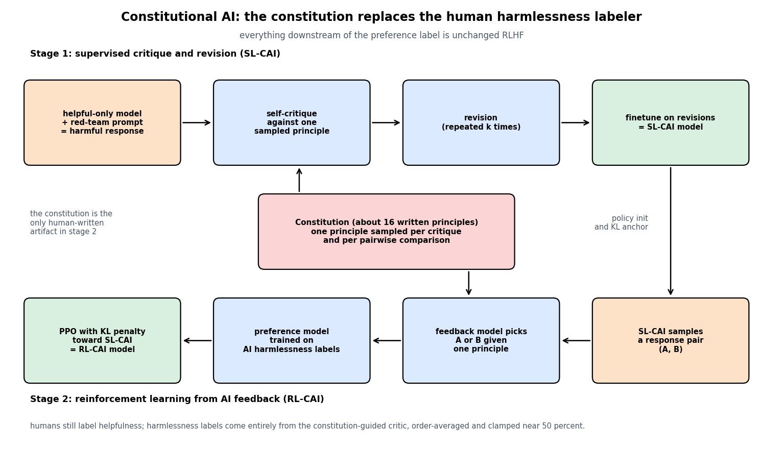
(5) Auditable Objective: a behavior change becomes a text edit to the constitution plus a rerun, rather than a new annotation guideline, a new labeler cohort, and a multi-week collection cycle.
(6) Bounded By The Critic: AI feedback inherits the critic’s position bias, self-preference, and capability ceiling, so it is strongest on axes where judging is easier than generating and weakest on novel or expert domains.

Two-lane pipeline diagram: the top lane runs left to right from a helpful-only model given a red-team prompt, to self-critique against a sampled principle, to revision repeated k times, to supervised finetuning that yields the SL-CAI model; the bottom lane runs right to left from SL-CAI sampling a response pair, to the feedback model choosing A or B given one principle, to a preference model trained on AI labels, to PPO with a KL penalty toward SL-CAI yielding RL-CAI; a constitution box between the two lanes sends arrows up to the critique step and down to the feedback model

Figure 1: The constitution is the only human-written artifact in the loop, and it touches the pipeline twice: once to steer self-critique and revision in the supervised stage, once to condition the critic’s pairwise judgments in the RL stage. Everything downstream of the label, the preference model and the KL-penalized policy update, is unchanged RLHF.

Three implementation details do most of the real work. First, order debiasing: language models judging “(A) or (B)” have a strong position preference, so each pair is scored twice with the options swapped and the two probabilities are averaged, which is cheap because compute is the only cost. Second, chain-of-thought judging with clamped probabilities: letting the critic reason before answering improves agreement with humans but produces near-deterministic 0.0 or 1.0 preferences, so the CAI work clamps the resulting probabilities into a narrow band around 50 percent to keep the preference model from training on overconfident targets. Third, a deliberately mixed label supply: RL-CAI does not eliminate humans, it reassigns them, training the preference model on human helpfulness comparisons alongside AI harmlessness comparisons, because harmlessness is the axis where labeling is unpleasant, high-variance, and easy to specify in writing. Empirically, the reported effect is not merely cheaper labels but a better trade-off, with RL-CAI models both more harmless and less evasive than an RLHF baseline, while the RLAIF study on summarization found AI-labeled and human-labeled policies statistically indistinguishable to human raters despite the critic agreeing with humans only about 78 percent of the time.

Mathematical Formulation:
$y^{(k+1)} \sim \pi_0(\cdot \mid x, y^{(k)}, c_k)$
$p_{\mathrm{AI}}(A \succ B) = \sigma(z_A - z_B)$
$\bar{p} = \frac{1}{2}\left(p_{AB} + 1 - p_{BA}\right)$
$\mathcal{L}_{\mathrm{PM}} = -\log \sigma\!\left(r_\phi(x,y_w) - r_\phi(x,y_l)\right)$
$J(\theta) = \mathbb{E}\left[r_\phi(x,y)\right] - \beta\,\mathrm{KL}\!\left(\pi_\theta \,\|\, \pi_{\mathrm{ref}}\right)$

Where:

$y^{(k)}$ is the response after $k$ revisions of the original answer to red-team prompt $x$ , and $\pi_0$ is the helpful-only model doing both the critique and the rewrite.
$c_k \sim \mathcal{C}$ is one principle sampled uniformly from the constitution $\mathcal{C}$ , typically around 16 short written rules.
$z_A$ and $z_B$ are the critic’s logits for the option tokens of the multiple-choice question, and $\sigma$ is the logistic function, so the label is a probability rather than a bit.
$p_{AB}$ and $p_{BA}$ are the probabilities assigned to the same candidate under the two presentation orders, and $\bar{p}$ is the order-debiased label actually stored.
$r_\phi$ is the preference model, $y_w$ and $y_l$ the winning and losing responses under $\bar{p}$ , and $\mathcal{L}_{\mathrm{PM}}$ the standard Bradley-Terry loss, unchanged from RLHF.
$\pi_\theta$ is the policy being optimized, $\pi_{\mathrm{ref}}$ is the frozen SL-CAI checkpoint, and $\beta > 0$ sets how far the policy may drift before the KL penalty dominates the reward.

Label Volume At A Fixed 100k USD Budget:
$N_{H} \approx 1.3 \times 10^{5}$
$N_{\mathrm{AI}} \approx 5.0 \times 10^{7}$
$N_{\mathrm{AI}} / N_{H} \approx 375$

The numbers assume a fully loaded cost near 0.75 USD per human comparison against roughly 0.002 USD for two short critic forward passes, which is why the same budget buys about 375 times more comparisons. Exact rates move with model size, context length, and vendor pricing, but the two orders of magnitude are robust, and they change what is even worth attempting: per-principle coverage sweeps, full relabeling after a constitution edit, and comparison sets larger than any human dataset ever collected. The binding constraint stops being annotation throughput and becomes critic quality plus reward-model overoptimization.

Left panel: log-log chart of labeling cost in dollars versus number of preference comparisons, with a steep line for human labels at 0.75 dollars each and a much lower line for AI labels at 0.002 dollars each, a horizontal line marking a 100000 dollar budget, and two marked crossing points at 133000 human labels and 50 million AI labels. Right panel: schematic scatter of harmlessness against helpfulness showing an evasive refusal model, a helpful-only RLHF model, an HH-RLHF model and an SL-CAI model lying on a dashed trade-off frontier, with RL-CAI plotted above and to the right of that frontier

Figure 2: Two different claims. On the left, the cost curve is the scaling argument, and at a fixed budget it is worth about 375 times more comparisons. On the right, the frontier shift is the alignment argument: human feedback tends to trade helpfulness against harmlessness, while self-critique plus AI harmlessness labels moves the operating point off that line instead of sliding along it. Right-panel positions are schematic illustrations of the reported qualitative result, not measured Elo scores.

Property	Classic RLHF	Generic RLAIF	Constitutional AI (RL-CAI)
Label source	Paid annotators following a private rubric	An off-the-shelf judge model with a prompt	Critic conditioned on one sampled principle from a published constitution
Cost and throughput	Roughly 1 USD per comparison, days to weeks per batch	Roughly 0.002 USD, limited only by inference capacity	Same as RLAIF, doubled for order swapping and chain-of-thought judging
Label form	Binary choice or coarse Likert rating	Soft probability from option logits	Soft probability, order-averaged and clamped near 50 percent
Auditability of the target	Low, values live in guidelines and labeler judgment	Medium, values live in an ad hoc judge prompt	High, values are a short versioned document you can diff
Human role	Label every comparison	Validate the judge on a held-out sample	Write and revise the constitution, still label helpfulness
Dominant failure mode	Annotator noise, sycophancy, length bias, slow iteration	Position and self-preference bias, silent capability ceiling	Behaviors no principle covers, and policy hacking of a critic that shares its blind spots

August 19, 2026

DL0174 Wide vs Deep LLM Architectures

Under a fixed parameter budget, what are the trade-offs between wider (more hidden dimensions, fewer layers) and deeper (more layers, narrower) Transformer architectures for LLMs, in terms of expressivity, training stability, and inference latency?

Answer

A decoder layer costs about $4d^{2}$ parameters in the attention projections and about $8d^{2}$ in the MLP, so a fixed budget pins the product $L d^{2}$ and the only remaining freedom is the aspect ratio $\rho = d/L$ . Cutting depth by 4x buys only 2x width, which is why the two axes are so asymmetric in practice. Depth buys serial computation: each layer is one more composition step, and multi-hop reasoning and compositional generalization improve with layers in a way that width cannot replicate. Width buys parallel capacity and hardware efficiency: larger GEMMs, higher arithmetic intensity, clean tensor-parallel sharding, and a smaller KV cache per token because the cache grows linearly in $L$ . Empirically the pretraining loss is remarkably insensitive to shape across the middle of the range, so the decision is usually settled by systems constraints rather than by quality. Depth is the axis that costs you latency and training stability, and width is the axis that costs you head redundancy, embedding budget, and eventual depth starvation.

(1) The Budget Is Quadratic In Width: the iso-parameter constraint is $L d^{2} = \mathrm{const}$ , so width is an expensive axis and depth is a cheap one. Doubling $d$ forces you to delete three quarters of the layers.
(2) Depth Is Serial Expressivity: a layer is one composition step, and tasks requiring $k$ chained inferences need enough layers to host them. Depth-efficiency saturates, though, with the useful depth for a given width growing only logarithmically in $d$ .
(3) Width Is Capacity And Throughput: knowledge storage tracks total parameters rather than shape, but wide layers give larger matrix multiplies, better MFU, and more heads per layer for parallel feature lookup.
(4) Depth Destabilizes Training: residual variance accumulates over $L$ branches, so deep stacks need $1/\sqrt{2L}$ output-projection init, Pre-LN or DeepNet-style residual scaling, and they show more loss spikes and attention rank collapse.
(5) Depth Is A Latency Multiplier: autoregressive decode pays a fixed per-layer serial cost (kernel launches plus two tensor-parallel all-reduces), so $L\tau$ adds directly to time per token even though total FLOPs are unchanged.
(6) Small Budgets Flip The Answer: the embedding matrix costs $Vd$ , which at a 128k vocabulary swamps a sub-billion model, so on-device work favors deep and thin shapes.

Log-log plot of model width d against number of layers L along the constant-parameter curve L times d squared equals 6.04e8, with three marked shapes: wide and shallow at 16 layers and width 6144 with aspect ratio 384, balanced at 36 layers and width 4096 with aspect ratio 114, and deep and thin at 64 layers and width 3072 with aspect ratio 48, plus region labels above the curve for exceeding the budget and below for budget unspent

Figure 1: Every shape on the curve costs the same parameters. The curve is a straight line in log-log space with slope $-1/2$ , which is the whole trade-off in one picture: width is quadratically expensive, so moving from 64 layers to 16 layers pays for only a 2x wider residual stream. Real production shapes cluster in the middle band, roughly $\rho$ between 60 and 160.

The stability side is where depth stops being free. In a Pre-LN residual stack the output is a sum of $L$ branch contributions, so without correction the variance entering the final norm grows roughly linearly in depth, gradients through the early layers get squeezed, and the effective learning rate per layer drifts as you add layers. The standard fixes are scaling the residual output projections by $1/\sqrt{2L}$ at init, DeepNet-style residual weighting for very deep stacks, and QK-norm to stop attention logits from drifting. Deep stacks also suffer token-uniformity (rank) collapse, where repeated pure attention drives representations toward a rank-one subspace and the MLPs plus residual path are what hold it off. Width has the opposite profile. Hyperparameter transfer across width is well understood through muP, so you can tune a small proxy model and reuse the learning rate, whereas transfer across depth needed its own theory. The failure mode of extreme width is not divergence but waste: many heads become redundant, the per-layer computation is over-provisioned relative to the number of serial steps available, and the model has no place to put a long chain of dependent inferences.

Mathematical Formulation:
$N \approx 12 L d^{2}$
$\rho = d / L$
$C_{\mathrm{kv}} = 2 L n_{\mathrm{kv}} d_{h} b$
$t_{\mathrm{dec}} \approx W / B + L \tau$

Where:

$N$ is the non-embedding parameter count, from $4d^{2}$ of attention projections plus $8d^{2}$ of MLP weights per layer (a SwiGLU MLP with hidden width $8d/3$ matches the same count).
$L$ is depth and $d$ the residual width; a fixed budget holds $L d^{2}$ constant, so 4x fewer layers buys 2x width.
$\rho$ is the aspect ratio, the single knob this question is really about. GPT-3 175B sits at $12288/96 = 128$ .
$C_{\mathrm{kv}}$ is KV-cache bytes per token, with $n_{\mathrm{kv}}$ key-value heads, head dimension $d_{h}$ , and $b$ bytes per element. Under GQA with a fixed head count it is proportional to $L$ alone.
$t_{\mathrm{dec}}$ is per-token decode latency, $W$ the weight bytes read per step, $B$ the achievable HBM bandwidth, and $\tau$ the fixed serial cost per layer from kernel launches and collective synchronization.
Because $W$ is set by the budget and not by the shape, the $W/B$ term is identical across shapes and only the $L\tau$ term differs.

Iso-Parameter Shapes At About 7.2B Non-Embedding Parameters:
$64 \times 3072^{2} \approx 6.04 \times 10^{8}$
$36 \times 4096^{2} \approx 6.04 \times 10^{8}$
$16 \times 6144^{2} \approx 6.04 \times 10^{8}$
$N \approx 12 \times 6.04 \times 10^{8} \approx 7.2 \times 10^{9}$

These three shapes are interchangeable on the training-cost sheet and nearly interchangeable on validation loss, yet they behave very differently in a serving stack. With GQA at 8 key-value heads and $d_{h} = 128$ in fp16, each layer stores 4 KiB per token, so the 64-layer shape carries 4x the KV cache of the 16-layer shape and supports a proportionally smaller batch at the same context length. On the latency side, a plausible tensor-parallel-8 deployment has roughly $\tau \approx 40$ microseconds per layer once you count two all-reduces plus launch overhead, which turns depth into 2.56 ms of pure serial cost at 64 layers against 0.64 ms at 16 layers, on top of an identical weight-read term.

Two panel chart: left panel shows stacked bars of per-token decode latency for the three iso-parameter shapes, each with an identical 0.90 millisecond weight-read term plus a serial per-layer term of 2.56, 1.44 and 0.64 milliseconds, giving totals of 3.46, 2.34 and 1.54 milliseconds and single-stream rates of 289, 427 and 649 tokens per second; right panel shows KV cache per 8192-token sequence of 2.0, 1.125 and 0.5 gibibytes for 64, 36 and 16 layers

Figure 2: Same parameters, same FLOPs, 2.2x difference in single-stream decode latency. The green weight-read term is fixed by the budget, so all of the spread comes from the $L\tau$ serial term. The right panel shows the second penalty of depth: KV cache is linear in $L$ , so the deep shape gives up 4x in memory per sequence and therefore in achievable batch size.

Property	Deep and thin (L=64, d=3072)	Balanced (L=36, d=4096)	Wide and shallow (L=16, d=6144)
Aspect ratio	48	114	384
Serial steps per token	64 composition steps, best compositional depth	36, enough for most multi-hop patterns	16, depth-starved on chained inference
GEMM shape	Many small matmuls, lower MFU in decode	Good balance on current accelerators	Few large matmuls, highest arithmetic intensity
KV cache per 8k sequence	2.00 GiB	1.125 GiB	0.50 GiB
Decode latency (TP=8 estimate)	3.46 ms per token, 289 tok/s	2.34 ms per token, 427 tok/s	1.54 ms per token, 649 tok/s
Parallelism fit	Pipeline stages are easy, but bubbles hurt small batches	Both TP and PP viable	Tensor-parallel friendly, hard to pipeline
Stability risk	Residual variance growth, loss spikes, rank collapse	Standard recipe suffices	Benign, muP transfers cleanly across width
Tied embedding cost (V=128k)	0.39B parameters	0.52B parameters	0.79B parameters

August 19, 2026

DL0173 Continuous vs Static Batching

How does continuous batching (iteration-level scheduling) in serving systems like vLLM and TGI differ from static request batching, and why does it improve GPU utilization under heterogeneous request lengths?

Answer

Static batching schedules at request granularity: the server collects up to $B$ requests, launches one generation loop, and that loop runs until the longest sequence in the group finishes. Every shorter sequence keeps holding its slot, its KV memory, and its lane in every matmul while emitting nothing useful, and a request that arrives one iteration after launch waits for the entire group to drain. Continuous batching, introduced as iteration-level scheduling in Orca and now the default in vLLM and TGI, moves the scheduling decision inside the loop: after every single forward pass the scheduler retires finished sequences, frees their KV blocks, and admits queued requests into the next pass. The batch is re-formed at each of the thousands of decode steps a request lives through, so the number of sequences actually producing a token stays pinned near the memory limit instead of decaying toward one. Because decoding is memory-bandwidth bound, that sustained batch size converts almost directly into tokens per second, which is why the win grows with the variance of output lengths.

(1) Scheduling Granularity: static batching makes one admission decision per batch, continuous batching makes one per forward pass, which is the entire conceptual difference.
(2) No Head-Of-Line Blocking: a finished sequence is evicted and a waiting request admitted on the next iteration, so queueing delay stops scaling with the longest generation in the current group.
(3) Padding Disappears: Orca’s selective batching batches the position-independent linear layers over flattened tokens and runs attention per sequence with variable-length kernels, so no pad tokens are ever computed.
(4) Paged KV Cache Makes Admission Cheap: PagedAttention allocates KV in fixed blocks rather than reserving a contiguous max-length buffer, so freed blocks immediately become admission capacity for a new prompt.
(5) Decode Is Bandwidth Bound: one decode step reads all model weights once regardless of $B$ , so a sustained batch amortizes that read across more tokens and lifts arithmetic intensity roughly linearly.
(6) The Cost Is Prefill Interference: admitting a long prompt injects a compute-heavy prefill into the loop and stalls every decoding sequence, producing inter-token latency spikes that chunked prefill was designed to remove.

Two stacked Gantt charts of four GPU batch slots across decode iterations for the same eight requests. The top chart shows static batching: the first four requests start together, three of them finish early and leave hatched idle slots until the longest request finishes at iteration 16, at which point the second group of four is admitted and finishes at iteration 23. The bottom chart shows continuous batching: as soon as a short request finishes, a queued request is admitted into the freed slot, so all eight requests complete by iteration 16 with far fewer idle cells.

Figure 1: The same eight requests and the same 50 sequence-iterations of useful decode work, scheduled two ways. Static batching spreads them over 23 iterations at 54% slot occupancy because the group cannot retire until its longest member does; continuous batching backfills every freed slot on the next iteration and finishes in 16 at 78% occupancy. The hatched cells are the entire cost of request-level scheduling: paid compute and reserved KV memory that produce no tokens.

The mechanics that make iteration-level scheduling possible are as important as the policy. A naive implementation would need all sequences in a batch to sit at the same generation position so the whole thing is one dense padded tensor, which is exactly why static batching pads. Selective batching breaks the batch apart: the QKV projections, MLP, and output head act on tokens independently, so they run over a flattened ragged tensor, while attention is dispatched per sequence with its own context length. PagedAttention then removes the second obstacle, memory fragmentation, by storing KV in fixed-size blocks (typically 16 tokens) that need not be contiguous, so a sequence grows block by block and a new arrival can be admitted whenever a handful of blocks are free. With both pieces in place, admission is bounded by free KV blocks rather than by a pre-declared batch shape, and the scheduler’s job becomes a per-iteration packing problem over a memory budget.

Why this shows up as GPU utilization is a roofline argument rather than a scheduling one. Generating one token for one sequence requires reading every weight from HBM, roughly 16 GB for an 8B model in fp16, but only about $2P$ FLOPs of arithmetic, so a batch of one runs at a tiny fraction of peak FLOPs and the GPU is idle waiting on memory. Adding sequences to the same forward pass reuses that single weight read for more tokens, so throughput climbs steeply until the KV-cache reads and finally the matmuls take over. Static batching’s effective batch size decays as its short members retire, so it spends most of its time in the low-intensity regime; continuous batching holds the batch near $B_{\max}$ and stays in the high-intensity regime. Reported end-to-end gains follow from this: Orca measured up to 36.9x throughput over a static FasterTransformer baseline at matched latency, and vLLM measured a further 2x to 4x from paged memory alone.

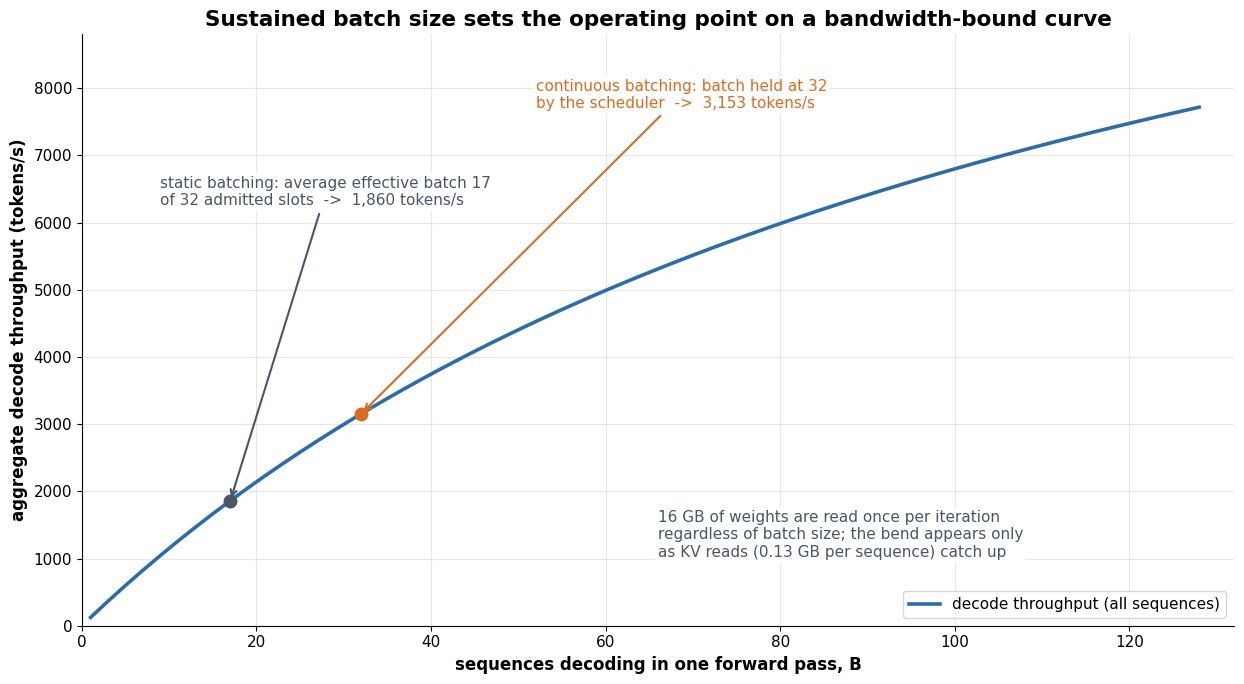
Line chart of aggregate decode throughput in tokens per second versus the number of sequences in the decode batch, from one to one hundred twenty-eight, for an eight-billion-parameter fp16 model with a one-thousand-token context on a two-terabyte-per-second GPU. The curve rises steeply and then bends as KV cache reads grow, with two marked points: an average effective batch of seventeen for static batching at about eighteen hundred tokens per second, and a sustained batch of thirty-two for continuous batching at about thirty-two hundred tokens per second.

Figure 2: Decode throughput against sustained batch size for an 8B fp16 model with 1K-token contexts on a 2 TB/s GPU. The curve is bandwidth-bound everywhere in this range, so throughput rises almost linearly at small $B$ and bends only as KV reads start to rival the 16 GB weight read. Continuous batching does not move the curve; it moves the operating point, from the average effective batch a draining static group achieves to the memory-limited maximum.

Mathematical Formulation:
$U_{\mathrm{static}} = \frac{\sum_{i=1}^{B} L_i}{B \, L_{\max}}$
$b_{\mathrm{kv}} = 2 \, n_l \, h_{kv} \, d_h \, s$
$t_{\mathrm{step}}(B) \approx \frac{2P + B \bar{L} b_{\mathrm{kv}}}{\mathrm{BW}}$
$\lambda(B) = B \, / \, t_{\mathrm{step}}(B)$
$B_{\max} = M_{\mathrm{free}} \, / \, (\bar{L} \, b_{\mathrm{kv}})$

Where:

$U_{\mathrm{static}}$ is the fraction of batch slot-iterations that produce a token under static batching, with $L_i$ the output length of request $i$ and $L_{\max} = \max_i L_i$ ; it is exactly 1 only when all lengths are equal.
$b_{\mathrm{kv}}$ is KV bytes per token, where $n_l$ is layers, $h_{kv}$ key/value heads (small under GQA), $d_h$ head dimension, $s$ bytes per element, and the leading 2 counts K and V.
$P$ is the parameter count, so $2P$ bytes is the fp16 weight read paid once per iteration regardless of $B$ , and $\mathrm{BW}$ is achievable HBM bandwidth.
$\bar{L}$ is the mean context length in the running batch and $B$ the number of sequences decoding in one forward pass.
$\lambda(B)$ is aggregate decode throughput in tokens per second; it is concave in $B$ because the KV term grows with $B$ while the weight term does not.
$M_{\mathrm{free}}$ is HBM left after weights and activations, so $B_{\max}$ is the admission ceiling the scheduler targets; the formula assumes $\bar{L}$ stays bounded, which it does not for sequences still growing.

Throughput At Two Operating Points (8B fp16, 1K context, 2 TB/s):
$\bar{L} \, b_{\mathrm{kv}} = 1024 \times 128\ \mathrm{KB} = 0.13\ \mathrm{GB}$
$t_{\mathrm{step}}(17) = 18.2 / 2000 = 9.1\ \mathrm{ms}$
$t_{\mathrm{step}}(32) = 20.2 / 2000 = 10.1\ \mathrm{ms}$
$\lambda(17) \approx 1870$
$\lambda(32) \approx 3170$

The byte totals are the 16 GB weight read plus $B \times 0.13$ GB of KV, divided by 2000 GB/s. Nearly doubling the sustained batch costs only 11% more time per step and yields 1.7x the tokens per second, which is the whole economic case for iteration-level scheduling: the extra sequences ride along in memory traffic that was already being paid.

Property	Static (request-level) batching	Continuous (iteration-level) batching	Continuous + chunked prefill
Scheduling unit	One whole generation loop per group	One forward pass	One forward pass with a token budget split across prefill and decode
Wait for a new arrival	Until the longest sequence in the current group finishes	One iteration, if KV blocks are free	One iteration, and its prefill is spread over several
Wasted compute	Pad tokens plus idle slots, growing with length variance	Near zero: ragged attention, no padding	Near zero, with better SM occupancy on decode-only steps
KV memory model	Contiguous buffer reserved for max length per slot	Paged blocks allocated on demand, freed on retirement	Same paged blocks, filled incrementally during prefill
Inter-token latency	Stable within a group, terrible queueing before it	Spikes whenever a long prompt is admitted	Bounded by the chunk size, at slightly higher TTFT
Dominant failure mode	Throughput collapse under heavy-tailed output lengths	KV exhaustion causing preemption and recompute thrash	Chunk size mistuned, trading TTFT against throughput

August 19, 2026

DL0172 Attention Collapse in Ultra-Deep Transformers

What actually causes attention collapse in ultra-deep Transformers with 100+ layers, uniform attention scores or rank degeneration, and how do register tokens, coupled attention, and SkipNet-style gated skipping address it?

Answer

Both phenomena are real, but they are not the same object and only one of them is the root cause. Rank degeneration is a property of the token matrix: after enough layers every row of $X^{(l)}$ converges to the same vector, so the representation is effectively rank-1 and no head can distinguish positions any more. Uniform attention scores are one route to that state but not a requirement, because every softmax attention map is row-stochastic, and a product of row-stochastic matrices contracts any mean-zero component of the token set by the second-largest eigenvalue at each step, even when each individual map looks sharp and interpretable. Dong et al. proved the sharper version of this: pure self-attention without residual connections or MLPs loses rank doubly exponentially in depth, so the residual stream, the FFN nonlinearity, and the normalization placement are the load-bearing defenses that let 100-layer stacks exist at all. A third, opposite pathology is attention entropy collapse, where rows become nearly one-hot as the spectral norm of the query-key map grows; that destroys training stability rather than smoothing representations, and it is the failure that spectral reparameterization targets. Register tokens, cross-layer attention coupling, and gated layer skipping each attack a different factor of the product that drives the representation toward rank-1.

(1) Two Different Objects: entropy of the attention rows measures how a layer mixes, while the rank of $X^{(l)}$ measures what survives after mixing. A model can have healthy per-layer entropy and still be rank-collapsed at layer 90.
(2) Doubly Exponential Rank Loss: for attention-only stacks the distance to rank-1 obeys a cubic recursion, so it is numerically zero within a handful of layers, not after 100.
(3) Non-Uniform Attention Still Collapses: because $A^{(l)}\mathbf{1} = \mathbf{1}$ , the all-ones vector is always a fixed point, and repeated application contracts everything else toward the Perron eigenvector.
(4) The Opposite Failure Mode: entropy collapse to near one-hot rows correlates with exploding query-key spectral norm and produces loss spikes; $\sigma$ Reparam bounds it by spectral-normalizing the logit map with a learned scalar.
(5) Register Tokens: a handful of learnable non-content tokens (typically 4 to 16) give softmax a place to dump probability mass, so content rows are not forced to spread uniformly and the emergent high-norm artifact tokens disappear.
(6) Coupled Attention: adding the previous layer’s raw logits to the current layer’s logits means the effective attention is no longer a fresh independent stochastic matrix per layer, which preserves diversity and gives gradients a direct path across depth.
(7) Gated Skipping: a SkipNet-style gate that drops a block reduces the effective mixing depth below the nominal $L$ , shortening the product of contraction factors and cutting sequential latency at the same time.

The reason a 100-layer Transformer is not already dead is that a residual block computes $X + \mathrm{Attn}(X)$ rather than $\mathrm{Attn}(X)$ . In path-decomposition terms, the identity path carries the full-rank input straight through, and only paths that traverse many attention modules are strongly contracted. The FFN nonlinearity adds a second defense by increasing the Lipschitz constant of the layer map away from a pure average, which is why the empirical decay of the distance to rank-1 in a working model looks geometric with a factor close to 1 instead of doubly exponential. The remaining problem at extreme depth is that these defenses only slow the contraction: with a per-layer factor of 0.95, a 120-layer stack still retains only about 0.2% of the initial token spread, which shows up as flat similarity matrices, near-duplicate hidden states in the last third of the network, and layers whose removal barely changes the loss.

Two panel chart. Left panel plots distance from rank-1 on a log scale against layer index for four settings: pure attention plunging off the chart by layer five, pre-LN residual only decaying geometrically to about 1e-4 at layer 120, residual plus MLP decaying to about 0.03, and a stabilized configuration staying above 0.5. Right panel plots attention entropy normalized by log N against layer index, showing one curve rising toward the uniform limit of 1.0, one curve falling toward zero labeled entropy collapse, and a stabilized curve staying inside a shaded healthy band.

Figure 1: The two collapse modes are measured on different axes. Left: rank degeneration is catastrophic for attention-only stacks, already below $10^{-8}$ by layer 5, and merely slow once residuals and FFNs are present. Right: entropy can fail in either direction, drifting up toward the uniform limit $\log N$ (over-smoothing) or down toward zero (entropy collapse and loss spikes), and a healthy deep model must stay in the band between them.

Mathematical Formulation:
$\mathrm{res}(X) = X - \mathbf{1}x^{\top}$
$\|\mathrm{res}(X^{l+1})\| \leq c\,\|\mathrm{res}(X^{l})\|^{3}$
$c^{1/2}\|\mathrm{res}(X^{L})\| \leq \left(c^{1/2}\|\mathrm{res}(X^{0})\|\right)^{3^{L}}$
$A^{(l)}\mathbf{1} = \mathbf{1}$
$\|A^{(l)}u\| \leq \lambda_2^{(l)}\|u\|$
$H(a_i) = -\sum_{j=1}^{N} a_{ij}\log a_{ij}$
$0 \leq H(a_i) \leq \log N$

Where:

$X^{(l)} \in \mathbb{R}^{N \times d}$ is the token matrix at layer $l$ , with $N$ tokens of width $d$ , and $L$ is the total depth.
$\mathrm{res}(X)$ is the distance to the nearest rank-1 matrix whose rows are all equal; $\mathbf{1}$ is the all-ones vector and $x$ the common row it would collapse to.
$c$ collects the head geometry, roughly $4\gamma\beta/\sqrt{d_{qk}}$ , where $\gamma$ and $\beta$ bound the value and query-key weight norms and $d_{qk}$ is the head dimension.
The cubic recursion compounds into a doubly exponential bound with exponent $3^{L}$ , which is why attention-only depth is hopeless while residual depth is merely expensive.
$A^{(l)} \in \mathbb{R}^{N \times N}$ is the row-stochastic attention map, so $\mathbf{1}$ is always its eigenvector with eigenvalue 1, and $u$ is any mean-zero deviation across tokens, $\mathbf{1}^{\top}u = 0$ .
$\lambda_2^{(l)}$ is the second-largest eigenvalue modulus of $A^{(l)}$ , strictly less than 1 whenever all entries are positive; the surviving spread after $L$ layers scales like $\prod_l \lambda_2^{(l)}$ .
$H(a_i)$ is the entropy of attention row $i$ ; the upper bound $\log N$ is the uniform row (maximal mixing) and 0 is the one-hot row (entropy collapse).

Collapse Speed, Two Regimes:
$0.9^{3^{5}} = 0.9^{243} \approx 7 \times 10^{-12}$
$0.95^{120} \approx 2.1 \times 10^{-3}$

The first line is the attention-only regime: five layers are enough to destroy the representation. The second is the realistic regime for a 120-layer residual stack with a mild per-layer contraction, and it is the number that motivates the three interventions. Register tokens change the geometry of each individual $A^{(l)}$ so that content rows keep structure instead of hedging uniformly; the attention sink observed in decoder-only LLMs, where the first token absorbs a large share of the mass, is the same phenomenon arising without being designed. Coupled attention changes the product itself, since adding the previous layer’s logits makes consecutive maps correlated rather than independent draws. Gated skipping changes the number of factors in the product, and it also attacks a separate ultra-deep pathology: under Pre-LN the output variance grows with depth, so late blocks approach the identity and contribute almost nothing, which means paying their latency buys no capacity.

Left to right architecture diagram of a deep Transformer segment. An input sequence box containing N content tokens plus R register tokens feeds block l minus 1, then block l, then a skip gate, then block l plus one, then an output box. A dashed arc above the stack shows attention logits from block l minus 1 being added to block l as coupled attention, an annotation above the input box explains that registers give softmax a non-content place to dump attention mass, and a routed path below the stack shows the gate bypassing block l plus one when its gate value is zero, reducing effective mixing depth.

Figure 2: Three interventions at three different levels of the same product. Registers reshape each individual attention map, coupled attention correlates consecutive maps so the stack stops re-averaging from scratch, and the skip gate removes factors entirely by lowering the effective depth. The residual stream and FFN remain the baseline defense underneath all three.

Property	Register tokens	Coupled attention	SkipNet-style gating
What it changes	The geometry of each single attention map	The correlation between consecutive maps	The number of maps in the product
Mechanism	Extra learnable non-content tokens absorb attention mass, so content rows need not spread uniformly	Pre-softmax logits of layer l minus 1 are added to layer l, giving a residual path through attention itself	A learned gate executes or bypasses a block per input, so effective depth is data dependent
Cost	Sequence grows to N plus R, so prefill cost grows quadratically in that length; registers are discarded at the head	Must retain the previous layer’s logit tensor, which is $O(hN^2)$ activation memory per block	Gate parameters plus non-differentiable routing, usually trained with a straight-through or RL estimator
Where it fails	Cannot be bolted on after pretraining, and too many registers waste context without adding capacity	Incompatible with kernels that never materialize the score matrix, so it fights FlashAttention-style fusion	Ragged per-example depth hurts batched throughput, and gates can collapse to always-on or always-off
Diagnostic it fixes	High-norm artifact tokens and noisy attention maps	Entropy drifting toward the uniform limit in late layers	Late blocks that behave as the identity and can be pruned for free

August 19, 2026