Tag: MLOps

DL0202 RL Production Recommendation

What are the challenges of using Reinforcement Learning in a production recommendation system, such as the YouTube home feed or Spotify’s carousels?

Answer

The hard part is almost never the learning algorithm. A production recommender is an off-policy problem with a combinatorial action space, a corrupted reward signal, and a closed feedback loop, and each of those violates an assumption that textbook RL takes for granted. You cannot explore freely on paying users, so the only training data is what yesterday’s serving policy logged, which makes importance weighting and its variance the central engineering problem rather than a footnote. The action is not one item but a slate of K items drawn from a catalogue of order $10^{8}$ , so enumerating a Q value per action is impossible and the policy must be factorized or decomposed. Finally, the reward you actually want, long-term satisfaction, arrives days after the action, and is confounded by position bias, seasonality, and the recommendations themselves.

(1) Off-Policy By Construction: training data comes from a logging policy $\beta$ , not from the policy you are optimizing, so every gradient needs an importance correction whose variance grows with the mismatch.
(2) Combinatorial Slate Actions: a page of $K$ items from $N$ candidates gives $\binom{N}{K}$ actions, forcing decompositions such as top-K correction or SlateQ‘s per-item value factorization.
(3) Reward Specification And Delay: clicks are immediate and gameable, retention is the real objective and is observed days later, so credit assignment spans sessions rather than steps.
(4) Feedback Loops And Non-Stationarity: the deployed policy shapes tomorrow’s training distribution, so a small early bias compounds instead of averaging out, and the catalogue and user base drift underneath the model.
(5) Offline Evaluation Is Unreliable: off-policy estimators are high variance on large action spaces, so offline value gains routinely fail to reproduce in an A/B test.
(6) Infrastructure Cost: you must log propensities at serving time, keep the randomization budget small, and still return a ranked page inside a tens-of-milliseconds latency budget.

Closed-loop diagram with four boxes in a row: serving policy pi-theta with retrieval and ranker over a 10^8 item catalogue, slate of K items shown to the user where position bias enters, logged feedback carrying the action, the propensity beta and a delayed reward, and off-policy training with IPS weights, clipping and top-K correction, with a return arrow deploying new policy weights back to serving

Figure 1: The loop is the problem. Supervised ranking treats the log as a fixed dataset, but here the policy under training generates its own future training distribution, so bias compounds across deployments and the reward attached to each logged action is both delayed and confounded by presentation.

The standard production recipe, popularized by YouTube’s top-K REINFORCE recommender, is to keep policy-gradient learning but reweight each logged trajectory by the ratio between the new policy and the logging policy. Two corrections then appear. The first is weight clipping, which caps the influence of any single log line and trades unbounded variance for a controlled downward bias. The second is the top-K correction factor, which accounts for the fact that the system shows $K$ slots rather than sampling one item, and which flattens the gradient on items the policy already places with near certainty. Both are variance-control devices, and understanding why they are needed is the difference between a candidate who has read the paper and one who has shipped the system.

Mathematical Formulation:
$J(\theta) = \mathbb{E}_{\tau \sim \pi_{\theta}}\left[\sum_{t=0}^{T} \gamma^{t} r_{t}\right]$
$w_t = \dfrac{\pi_{\theta}(a_t \mid s_t)}{\beta(a_t \mid s_t)}$
$\tilde{w}_t = \min(w_t, c)$
$\lambda_K(s_t, a_t) = K\left(1 - \pi_{\theta}(a_t \mid s_t)\right)^{K-1}$
$\hat{g} = \sum_{t} \tilde{w}_t\, \lambda_K\, R_t\, \nabla_{\theta} \log \pi_{\theta}(a_t \mid s_t)$
$\mathrm{ESS} = \dfrac{\left(\sum_i w_i\right)^{2}}{\sum_i w_i^{2}}$

Where:

$J(\theta)$ is the expected discounted return of the target policy over a user trajectory $\tau$ , with discount $\gamma \in (0,1]$ and per-step reward $r_t$ .
$s_t$ is the user state (interaction history and context), $a_t$ the item actually shown and logged, and $R_t$ the return following that action.
$\pi_{\theta}$ is the target policy and $\beta$ the logging (behavior) policy; $w_t$ is their ratio, and it is undefined wherever $\beta(a \mid s) = 0$ .
$c$ is the clipping threshold; $\tilde{w}_t$ is the truncated weight, which is biased but bounded.
$\lambda_K$ is the top-K correction for showing $K$ slots instead of one; it tends to $K$ for rare items and to $0$ as $\pi_{\theta}(a \mid s)$ approaches $1$ .
$\mathrm{ESS}$ is the effective sample size over $i \in \{1,\ldots,N\}$ logged records, and it is the number that decides whether a 10M-row log is really 10M rows.

Log-scale line chart of effective sample size fraction versus policy mismatch sigma, showing an unclipped importance-sampling curve collapsing from near one to about one thousandth as sigma grows to three, a curve clipped at one hundred decaying more slowly, and a curve clipped at ten still retaining several percent, with an annotation marking that at sigma equal to two the unclipped estimator retains about two percent of the logged rows

Figure 2: Why off-policy learning is a variance problem before it is an optimization problem. As the target policy drifts from the logging policy, the effective sample size of the log collapses exponentially, so a huge log can carry the statistical weight of a small one. Clipping restores usable sample size at the price of a systematic downward bias on exactly the actions the new policy likes most.

This is also why the choice between supervised ranking, a contextual bandit, and full sequential RL is a real design decision rather than a question of ambition. A bandit captures most of the exploration benefit with a single-step correction and no long-horizon credit assignment, and it is what Spotify’s explainable-recommendation work uses for carousel and explanation selection. Full RL earns its cost only when an action genuinely changes the future state, for example when promoting a new creator today changes what the user is willing to watch next month.

Property	Supervised ranker	Contextual bandit	Full sequential RL
Objective	Predict the immediate label, click or watch probability	Maximize immediate reward under uncertainty	Maximize discounted return across future sessions
Data required	Logged impressions and labels only	Logged action plus its propensity	Full trajectories with propensities and delayed rewards
Correction needed	None in principle, though position bias still needs debiasing	Single-step IPS or doubly robust	Per-step IPS, clipping, top-K factor, bootstrapped value targets
Exploration cost	None, and therefore no counterfactual coverage	Small randomized slot, epsilon-greedy or Thompson sampling	Randomization plus pessimism penalties for out-of-support actions
Dominant failure	Myopic optimization that rewards clickbait	No credit for downstream session value	Variance explosion offline and feedback-loop drift online

August 21, 2026

DL0201 Pretraining Loss Spike Debugging

During pretraining of a 100B parameter model on a large GPU cluster, you suddenly see loss spikes. How do you debug this, and is it a data issue, a learning-rate problem, or hardware failure?

Answer

All three causes are real at this scale, and they leave different fingerprints, so the answer is a triage order rather than a guess. Run the checks in order of cost: first the numerics and per-rank logs you already have on disk (NaN or Inf, one data-parallel rank far from the mean loss, XID or ECC events, NCCL timeouts), then the optimizer traces (global gradient norm, Adam update ratio, maximum attention logit, output logit magnitude), and only then the data, which is proven guilty only by replaying the exact batch from the pre-spike checkpoint. The shape of the curve already narrows the space: a single sharp spike that recovers within a few thousand steps is usually a batch-times-model-state interaction, a slow creeping divergence preceded by growing logits is a learning-rate or numerics problem, and an instant jump to NaN with a stalled step time is hardware. The industry-standard mitigation for the first case is the one PaLM reported: rewind to a checkpoint roughly 100 to 200 steps before the spike and skip a few hundred batches, which removes the spike even though the same data is harmless from a different model state. That asymmetry is the single most important fact in this debugging problem, because it means “the data was bad” is almost never the correct conclusion on its own.

(1) Read The Shape First: recoverable spike, creeping divergence, and hard fault are three distinct signatures, and each maps to a different subsystem.
(2) Cheapest Check First: numerics and per-rank divergence cost nothing to inspect, optimizer traces cost one dashboard query, and a batch replay costs about one node-hour.
(3) Never Trust The Global Loss: with 512 data-parallel ranks a single sick rank moves the average by a fraction of a percent, so log per-rank loss and gradient-norm maxima, not just the mean.
(4) Silent Data Corruption Has No NaN: a degrading GPU can return wrong arithmetic with no error flag, so keep a bitwise-reproducibility canary that reruns one batch on two hosts and compares.
(5) Data Is Guilty Only On Replay: rerun batch $b_s$ from the checkpoint at step $s-1$ on a fresh replica; if the spike does not reproduce, the batch is not the cause.
(6) Skip-And-Resume Versus Config Change: rollback is right for isolated spikes, but recurring spikes plus growing attention logits mean you must pay for QK-norm, z-loss, a lower peak learning rate, or fp32 optimizer state.

Two-row by three-column chart grid. Top row shows training loss versus step for three cases: a single sharp spike at step 9000 that recovers to trend, a creeping divergence starting near step 11500 that never returns, and a curve that ends abruptly at step 15000 with a NaN marker. Bottom row shows the corresponding global gradient norm on a log scale with a clipping threshold line at 1.0: a single narrow 15x spike, a gradient norm that creeps up for two thousand steps before the loss moves, and a flat trace that terminates in an infinite value.

Figure 1: The same symptom, three diseases. Case A is a recoverable spike whose gradient norm spikes for a handful of steps and then returns, case B is a creeping divergence in which the gradient norm rises for roughly 2,000 steps before the loss visibly moves, and case C is a hard fault with no precursor at all. Note that gradient clipping at 1.0 caps the applied update but does not hide the raw norm, which is exactly why the raw norm must be logged.

The mechanism behind case B is worth being precise about, because it is the one people misdiagnose as bad data. As training proceeds, attention logits $q_i^\top k_j / \sqrt{d_h}$ can grow without bound; the softmax saturates, one head collapses onto a single position, and the gradient through that head becomes both tiny and extremely sharp. In parallel, the output logits drift so that $\log Z$ wanders, which makes the cross-entropy surface stiff in a direction the optimizer cannot see from the loss value alone. Case A has a different mechanism: in bf16 or when optimizer state is stored in low precision, the Adam second moment for a rarely-activated parameter block (embeddings for rare tokens are the classic example) can decay toward the epsilon floor, after which one moderate gradient produces an update whose effective step size is orders of magnitude larger than intended. The debugging pipeline is therefore always the same: detect → localize → replay → mitigate, with instrumentation decided before the run rather than after the first spike.

Mathematical Formulation:
$\ell_t > \mu_{t-W:t} + 3\,\sigma_{t-W:t}$
$\theta_{t+1} = \theta_t - \eta_t \dfrac{\hat m_t}{\sqrt{\hat v_t} + \epsilon}$
$r_t = \dfrac{|\hat m_t|}{\sqrt{\hat v_t} + \epsilon}$
$r_{\max} \approx \dfrac{1-\beta_1}{\sqrt{1-\beta_2}}$
$s_{ij} = q_i^\top k_j / \sqrt{d_h}$
$\mathcal{L} = \mathcal{L}_{\mathrm{CE}} + \alpha (\log Z)^2$

Where:

$\ell_t$ is the training loss at step $t$ , and $\mu$ and $\sigma$ are the mean and standard deviation over a trailing window of $W$ steps (a few hundred works well); this is the spike detector that should fire an alert, not a human eye on a dashboard.
$\theta_t$ are the parameters, $\eta_t$ the scheduled learning rate, and $\hat m_t$ and $\hat v_t$ the bias-corrected first and second Adam moments with decays $\beta_1$ and $\beta_2$ .
$r_t$ is the update ratio, the per-block quantity to log alongside the gradient norm, because it exposes the actual step size the optimizer is taking rather than the size of the gradient.
$r_{\max}$ is the ratio a single outlier gradient can produce, roughly $0.1/\sqrt{0.05} \approx 0.45$ for $\beta_1 = 0.9$ and $\beta_2 = 0.95$ ; this bound holds only while $\sqrt{\hat v_t}$ dominates $\epsilon$ , and it is epsilon underflow that breaks it.
$s_{ij}$ is the pre-softmax attention logit for query $i$ and key $j$ with head dimension $d_h$ ; tracking $\max_{ij} |s_{ij}|$ per layer is the earliest available warning of the creeping-divergence mode.
$Z = \sum_{v=1}^{V} \exp(z_v)$ is the softmax partition function over vocabulary size $V$ , and $\alpha$ is the z-loss coefficient (commonly $10^{-4}$ ) that pins $\log Z$ near zero at negligible quality cost.

The $r_{\max} \approx 0.45$ bound is the reason “one weird document blew up the run” is usually wrong: with healthy second moments, Adam already damps a single 30x outlier gradient to less than a normal step. What actually hurts is a sequence of correlated large gradients, or a block whose $\hat v_t$ has collapsed so that the denominator is dominated by $\epsilon$ . That distinction determines the fix: correlated gradients are a data-ordering and learning-rate problem, while a collapsed second moment is a precision problem solved by keeping optimizer state in fp32 and raising $\epsilon$ .

Left-to-right triage diagram. A trigger box for a detected loss spike fans out to three ordered check boxes: numerics and per-rank divergence, optimizer signals such as gradient norm and maximum attention logit, and a replay of the offending batch from the previous checkpoint. Each check has a yes branch to an evidence box listing concrete symptoms, and each evidence box points to a verdict box: hardware, learning rate and numerics, or data crossed with model state. Vertical clean arrows connect check one to check two and check two to check three.

Figure 2: The triage order that makes this question answerable in an interview. The three branches are ordered by cost per bit of information, not by likelihood, and the replay step is what separates a genuinely corrupt shard from a batch-times-state interaction that a 400-batch skip will silently fix.

Signal	Data and model state	Learning rate and numerics	Hardware and interconnect
Loss shape	Sharp isolated spike, recovers to trend within a few thousand steps	Repeated spikes of growing size, or a divergence that never recovers	Instant NaN or Inf, or a flat line while step time stalls
Gradient norm	One narrow burst of a few steps, clipping engages briefly	Slow upward drift over thousands of steps, clipping engages permanently	Jumps straight to Inf, or becomes exactly zero on one rank
Per-rank pattern	Elevated on the ranks holding the offending microbatches only	Uniform across all ranks, since the cause is the shared update	One rank or one host is an extreme outlier, or a canary mismatches bitwise
Replay test	Reproduces from the same checkpoint, disappears from a different one	Reproduces from any nearby checkpoint with the same schedule	Does not reproduce on a healthy node with identical inputs
Corroborating logs	Sample dump shows repeated n-grams, a truncated shard, or non-text bytes	Max attention logit and update ratio rising, parameter norm inflating	XID or ECC entries, NCCL timeouts, thermal throttling, link flaps
First mitigation	Rewind about 200 steps, skip 200 to 500 batches, then dedup or drop the shard	Lower peak LR, extend warmup, add QK-norm and z-loss, keep fp32 optimizer state	Fence the host, restore the last checkpoint, rerun on a spare node

The operational context matters for how much of this you should automate. Meta reported 419 unexpected interruptions during Llama 3 405B pretraining, with roughly 78% traced to hardware, which means at 100B scale a fault-driven anomaly is not an exotic event but a weekly one. That argues for treating spike response as a control loop: an automatic detector on the trailing-window rule, automatic checkpoint retention dense enough to rewind 200 steps, automatic host fencing on XID events, and a human decision only for the residual class where the numerics themselves are unstable.

August 21, 2026

DL0200 BERT GPU Underutilization

What can cause a BERT-based model to struggle with GPU underutilization, how do you detect CPU-side preprocessing bottlenecks, and what optimizations (pinned memory, ONNX export, TensorRT, INT8 quantization) would you recommend?

Answer

A BERT forward pass at batch 32 and sequence length 128 is a few milliseconds of dense GEMM work, so the GPU is almost never the slow part of a badly performing BERT service. Underutilization comes from three separable causes: the host-side pipeline (Python tokenization, collation, and synchronous host-to-device copies that block the training or serving loop), wasted GPU work (padding every request to max_length, batch size 1 traffic, or fragmented small kernels whose launch overhead exceeds their compute), and framework overhead (eager-mode PyTorch dispatching hundreds of tiny kernels per layer instead of fused ones). Detection is a matter of separating those causes rather than staring at the single nvidia-smi utilization number, which reports only whether any kernel was resident during a sampling window and happily shows 90% while the SMs are mostly idle. The fix ladder is ordered by cost: first hide the host work with fast tokenizers, multiple dataloader workers, pinned memory plus non_blocking copies and prefetch; then remove padding waste with length bucketing and dynamic batching; then export to ONNX for graph fusion and constant folding; then build a TensorRT engine in FP16; and only last apply INT8 post-training quantization, which is the only step in the list that can change your accuracy.

(1) Host-Bound Pipeline: a Python BertTokenizer plus per-batch collation can cost 15-25 ms while the forward pass costs 6 ms, so a serial loop pins utilization near 25% no matter how fast the GPU is.
(2) Synchronous Copies: a transfer from pageable host memory cannot be overlapped with compute, because the driver must stage it through an internal pinned buffer; pinned memory plus non_blocking=True is what makes DMA overlap legal.
(3) Padding Waste: attention cost scales as $O(L^2)$ , so padding a batch whose mean length is 27 tokens out to 128 burns roughly 79% of the tokens on [PAD], which looks like high utilization and low throughput.
(4) Kernel Launch Overhead: eager BERT-base issues on the order of a thousand kernels per forward pass; at batch 1 the launch and layout overhead, not the math, sets latency.
(5) Detection By Elimination: loop over one cached pre-tokenized tensor. If throughput jumps, the bottleneck was host-side; if it does not, profile kernels with Nsight Systems and look at gaps between them.
(6) Optimize In Cost Order: dataloader and padding fixes are free and safe, ONNX and TensorRT FP16 are numerically near-lossless, and INT8 is the only step that requires a calibration set and an accuracy regression gate.

Two stacked timelines in milliseconds. The upper pair shows a serial dataloader where the CPU tokenizes for 18 ms while the GPU row is idle, then the GPU computes for 6 ms while the CPU waits, repeating so the GPU is idle three quarters of the time. The lower pair shows three CPU worker lanes tokenizing in staggered 18 ms windows offset by 6 ms each, after an 18 ms prefetch warm-up, feeding a GPU row of back-to-back 6 ms forward passes with no gaps.

Figure 1: The same model and the same GPU, two pipelines. In the serial loop the GPU waits for tokenization and the utilization ceiling is $6/(18+6) = 25\%$ . With three prefetching workers writing into pinned buffers, host work is fully hidden behind compute after an 18 ms warm-up and the GPU runs back to back. No kernel was made faster here; only the schedule changed.

How To Detect A Host-Side Bottleneck: start by distrusting the utilization percentage. nvidia-smi samples whether at least one kernel was resident, not how many SMs were busy, so query DCGM fields such as SM activity and SM occupancy, or run nvidia-smi dmon and watch the memory-controller column: a host-bound job shows low SM activity and near-zero copy activity in the gaps. Then run the decisive experiment, which takes ten minutes: tokenize one batch once, keep it on the device, and loop the forward pass. That measures your true kernel-only throughput, and the gap between it and end-to-end throughput is exactly your host overhead. Confirm the cause with torch.profiler (look for aten::copy_, cudaStreamSynchronize, and dataloader wait time) or an Nsight Systems timeline, where a host-bound run appears as short kernel clusters separated by long empty stretches on the CUDA stream. Common culprits found this way: the slow Python tokenizer instead of the Rust BertTokenizerFast, num_workers=0, tokenizing inside the request handler on the same thread that owns the GPU, a stray .item() or .cpu() inside the loop forcing a sync every step, and logging metrics per step.

Mathematical Formulation:
$U_{\mathrm{serial}} = \frac{t_{\mathrm{gpu}}}{t_{\mathrm{cpu}} + t_{\mathrm{gpu}}}$
$U_{\mathrm{ovl}} = \frac{t_{\mathrm{gpu}}}{\max(t_{\mathrm{cpu}}/W,\; t_{\mathrm{gpu}})}$
$C \propto B\,(L^2 d + L d^2)$
$w = 1 - \bar{L}/L_{\max}$

Where:

$U$ is the fraction of wall-clock time the GPU spends executing kernels, capped at 1, with $U_{\mathrm{serial}}$ for a blocking loop and $U_{\mathrm{ovl}}$ for an overlapped prefetch pipeline.
$t_{\mathrm{cpu}}$ is per-batch host time (tokenize, collate, copy) and $t_{\mathrm{gpu}}$ is per-batch device time for the forward, or forward plus backward when training.
$W$ is the number of dataloader workers or preprocessing processes; overlap only holds if their output lands in pinned memory and the copy is issued as non_blocking.
$C$ is the dominant FLOP count per batch with $B$ the batch size, $L$ the padded sequence length, and $d$ the hidden width; the $L^2 d$ term is attention and the $L d^2$ term is the projections and feed-forward.
$w$ is the fraction of computed tokens that are padding, with $\bar{L}$ the mean true length and $L_{\max}$ the padded length; $w$ understates the true waste whenever the $L^2$ term dominates.

Worked Numbers For One Batch:
$U_{\mathrm{serial}} = \frac{6}{18 + 6} = 0.25$
$U_{\mathrm{ovl}} = \frac{6}{\max(18/3,\; 6)} = 1.0$
$w = 1 - \frac{27}{128} = 0.79$

Three workers are enough to hide 18 ms of host work behind a 6 ms forward pass, and the same arithmetic tells you when adding workers stops helping: once $t_{\mathrm{cpu}}/W$ drops below $t_{\mathrm{gpu}}$ , extra workers only add memory pressure and page-cache churn. The padding figure is the other half of the story. Sorting a serving queue by length into buckets, or using dynamic padding to the longest member of each batch, typically recovers most of that 79% at zero accuracy cost, and it is strictly better than buying a larger GPU to compute attention over [PAD] tokens faster.

Bar chart of throughput in sequences per second for five BERT-base inference configurations at batch 32 and sequence length 128 on a single mid-range GPU: PyTorch eager FP32 with a serial tokenizer at 210, PyTorch eager FP32 with three workers and pinned memory at 320, ONNX Runtime FP32 with a fused graph at 480, TensorRT FP16 at 1150, and TensorRT INT8 with post-training calibration at 1900.

Figure 2: An illustrative optimization ladder for BERT-base at batch 32, sequence 128, on one mid-range GPU. Each rung removes a different bottleneck: host stalls first, then kernel launch and layout overhead through graph fusion, then arithmetic precision. Only the last rung can move your evaluation metric, which is why it ships behind an accuracy gate.

Property	PyTorch eager	ONNX Runtime	TensorRT (FP16 / INT8)
Graph optimization	None by default; op-by-op dispatch	Constant folding, LayerNorm and GELU fusion, attention fusion	Full autotuned kernel selection plus fused multi-head attention
Variable sequence length	Free; any shape runs	Dynamic axes supported, some re-optimization per new shape	Needs declared optimization profiles; shapes outside them fail or fall back
Build and deploy cost	Zero; ship the checkpoint	One export step, portable artifact	Minutes of engine build, plus a calibration pass for INT8
Portability	Runs anywhere PyTorch runs	CPU, GPU, and other execution providers	Engine is tied to GPU architecture and TensorRT version
Accuracy risk	Baseline	Numerically equivalent in FP32	FP16 usually within noise; INT8 needs a regression gate
Dominant failure mode	Launch overhead and host stalls dominate at small batch	Unsupported op forces a subgraph back to a slow path	Engine rebuild on driver or hardware change; activation outliers break INT8

Code Implementation:

# 1) hide host work: fast tokenizer, workers, pinned memory, prefetch
from transformers import AutoTokenizer
tok = AutoTokenizer.from_pretrained("bert-base-uncased", use_fast=True)

def collate(batch):
    # dynamic padding to the longest item, not to max_length
    return tok([b["text"] for b in batch], padding=True,
               truncation=True, max_length=128, return_tensors="pt")

loader = torch.utils.data.DataLoader(
    ds, batch_size=32, collate_fn=collate,
    num_workers=4, pin_memory=True, persistent_workers=True,
    prefetch_factor=4)

for batch in loader:
    batch = {k: v.to("cuda", non_blocking=True) for k, v in batch.items()}
    with torch.autocast("cuda", dtype=torch.float16):
        out = model(**batch)      # no .item() / .cpu() inside the loop

# 2) measure kernel-only throughput to prove where the time goes
cached = {k: v.cuda() for k, v in collate(ds[:32]).items()}
torch.cuda.synchronize(); t0 = time.perf_counter()
for _ in range(200):
    with torch.no_grad(), torch.autocast("cuda", dtype=torch.float16):
        model(**cached)
torch.cuda.synchronize()
print("device-only seq/s:", 200 * 32 / (time.perf_counter() - t0))

# 3) export and build: ONNX -> TensorRT with dynamic shape profiles
# torch.onnx.export(model, tuple(cached.values()), "bert.onnx",
#                   dynamic_axes={"input_ids": {0: "B", 1: "L"}}, opset_version=17)
# trtexec --onnx=bert.onnx --fp16 --int8 --calib=calib.cache \
#         --minShapes=input_ids:1x16 --optShapes=input_ids:32x128 \
#         --maxShapes=input_ids:64x256 --saveEngine=bert.plan

August 21, 2026

DL0194 Sensor Degradation Feature Extractor

How do you detect and handle sensor degradation (lens distortion, rain noise, sensor misalignment) dynamically within a deep feature extractor pipeline, for a production perception stack such as a robotaxi’s camera-LiDAR fusion model or a Valeo-style surround-view ADAS?

Answer

Degradation is not handled by making the backbone bigger. It is handled by a cheap monitoring path that runs beside the feature extractor and a policy layer that changes how the extractor’s outputs are consumed. Three monitor families are affordable per frame: referenceless image-quality and soiling heads on the raw or early-feature tensor, feature-space drift statistics such as a Mahalanobis distance between the current channel-mean vector and the training reference, and geometric self-consistency residuals such as cross-sensor reprojection error, which is the only signal that separates a genuine extrinsic shift from bad weather. Detection alone is worthless, so those signals drive three mitigations: a quality gate that reweights per-sensor features before fusion, FiLM-style conditioning that lets the shared trunk adapt its normalization to the measured degradation, and an operational-design-domain (ODD) fallback that reduces speed, disables a fused output, or triggers a wiper and an online extrinsic re-estimation. The pipeline therefore reads capture → ISP → undistort → backbone → gate → fusion → heads, with the monitors tapping the first three stages and writing only into the gate.

(1) Separate Detection From Correction: a small monitor head that answers “how bad is this input” is far easier to train and validate than a backbone expected to be silently invariant to everything. It also gives you an auditable signal to log.
(2) Three Complementary Signals: pixel-level quality catches soiling and droplets, feature drift catches global appearance shift like rain veiling or blooming, and reprojection residuals catch calibration error. No single one covers all three failure classes.
(3) Geometry For Geometry Faults: a 0.5 degree extrinsic yaw drift leaves every image looking perfectly clean, so appearance-based monitors are blind to it; only cross-sensor residuals or photometric alignment expose it.
(4) Gate The Fusion, Not The Backbone: down-weighting a corrupted branch with normalized weights $w_m$ is a one-line change at inference and needs no retraining, whereas swapping backbone weights per weather condition doubles the validation surface.
(5) Train For Dropout, Not Just For Rain: corruption augmentation plus random modality dropout is what makes a gated fusion model usable when a branch is masked, otherwise the fused head has never seen a zeroed input.
(6) Absolute Scores Plus An Abstention Path: a softmax gate can only express relative trust, so a separate calibrated absolute quality score must be able to declare that all sensors are bad and hand control to the ODD layer.

Architecture diagram with three sensor lanes for front camera, side camera, and LiDAR, each passing through a per-sensor encoder and a quality head, all feeding a tall degradation gate box that computes fusion weights and FiLM conditioning, then a feature fusion block, then detection heads and a degradation-state and fallback block, with an online monitor box at the bottom sending dashed arrows to the gate and back to the encoder for recalibration

Figure 1: The monitors sit outside the critical path and write only into the gate. An alarm changes the fusion weight $w_m$ , the FiLM conditioning, and the declared ODD, but it never edits backbone weights at runtime, which keeps the deployed model bit-identical and the failure behaviour testable.

Each monitor has a different latency and a different false-alarm profile. The soiling and quality head is a per-tile classifier over an early feature map, typically under 1 ms on an embedded accelerator, and it is the only monitor fast enough to drive a physical actuator such as a nozzle or a heater. Feature drift is computed from the channel means of a mid-level tensor against a reference mean and covariance collected on clean data, then smoothed by a CUSUM accumulator so that a single dark frame does not raise an alarm while a sustained shift does within a few frames. Reprojection residuals need matched features across overlapping fields of view or LiDAR points projected into the image, so they run at a lower rate over a sliding window of several seconds, which is acceptable because extrinsic drift from thermal expansion or a curb strike is either slow or a step change that persists. Lens distortion sits between these cases: an intrinsics change makes straight lines curve and inflates residuals even for a single camera, and the correct response is to re-estimate the undistortion look-up table rather than to touch the network, because a CNN trained on rectified images treats a mis-rectified frame as out-of-distribution geometry.

Two stacked time-series panels over 300 camera frames. The top panel shows feature-drift distance rising from about 1.15 to 3.5 during a shaded rain burst between frames 90 and 170 while the reprojection residual stays near 0.35 pixels, then a second shaded region after frame 200 where the reprojection residual steps to about 2.5 pixels while feature drift stays low, with a dashed one-pixel residual threshold. The bottom panel shows the CUSUM statistic on feature drift staying at zero, then sawtoothing above a threshold of five during the rain burst with alarm markers.

Figure 2: The two monitors have orthogonal signatures. Rain moves the feature-drift statistic and leaves the reprojection residual untouched, while a mount shift moves the residual by 2.5 px without disturbing appearance statistics at all. Reading only one monitor guarantees you misdiagnose one of the two faults.

Quality-Gated Fusion:
$q_m = \sigma(g_{\phi}(F_m))$
$\hat{F}_m = \gamma(q_m) \odot F_m + \beta(q_m)$
$w_m = \frac{\exp(a_m + \log q_m)}{\sum_j \exp(a_j + \log q_j)}$
$F = \sum_m w_m \hat{F}_m$

Where:

$F$ is the fused feature tensor consumed by the task heads, and $F_m$ is the raw feature map of sensor $m$ , with $\hat{F}_m$ its degradation-conditioned version.
$q_m \in [0,1]$ is the absolute quality score produced by a small monitor head $g_{\phi}$ with logistic output $\sigma$ ; it is supervised by synthetic corruption labels and calibrated on held-out real degraded clips.
$\gamma(\cdot)$ and $\beta(\cdot)$ are the FiLM scale and shift vectors, and $\odot$ is channel-wise multiplication.
$a_m$ is a content-dependent attention logit from the ordinary fusion module, so the gate combines what is informative with what is trustworthy.
$w_m$ sums to 1 over sensors $m$ , which is why a low but uniform $q$ across all sensors must be caught by the raw $q_m$ values rather than by the weights.

Runtime Degradation Monitors:
$d_t^2 = (\mu_t - \mu_0)^{\top} \Sigma_0^{-1} (\mu_t - \mu_0)$
$S_t = \max(0, S_{t-1} + d_t - k)$
$r_{ij} = \| u_i - \pi(T_{ij} X_j) \|_2$

Where:

$d_t$ is the Mahalanobis drift at frame $t$ between the current channel-mean vector $\mu_t$ of a mid-level feature map and the clean-data reference $\mu_0$ with covariance $\Sigma_0$ .
$S_t$ is the CUSUM statistic with slack $k$ , which is set just above the clean-condition mean of $d_t$ ; an alarm is raised when $S_t > h$ and $S_t$ is then reset to 0.
$r_{ij}$ is the reprojection residual in pixels for correspondence $(i,j)$ , where $u_i$ is the observed image point, $X_j$ the 3D point from LiDAR or a second camera, $T_{ij}$ the extrinsic transform, and $\pi$ the projection using current intrinsics.
A robust percentile of $r_{ij}$ above roughly 1 px sustained over a window indicates extrinsic or intrinsic drift rather than matching noise, and triggers online recalibration.

The handling policy has to be trained for, not bolted on. A gate that can zero a camera branch is only safe if the fused head saw randomly dropped modalities and heavy corruption augmentation during training, otherwise masking a branch pushes the fusion layer into a region it never visited and accuracy collapses harder than with the corrupted input left in place. Augmentation alone is also insufficient, because it buys average-case robustness while a gate buys graceful worst-case behaviour: at high rain severity the model that can lean on LiDAR keeps far more of its mAP than the model that must average a clean point cloud with a veiled image. The cost is roughly one mAP point in clean weather, from the gate occasionally distrusting a good camera, plus the engineering burden of calibrating $q_m$ so that the gate does not permanently learn to ignore a sensor after a single bad deployment week.

Line chart of mAP versus rain and spray severity from level zero to five for three configurations: a clean-trained fusion baseline falling from 58 to 19, the same model with corruption augmentation falling from 58 to 31, and augmentation plus quality gating with LiDAR fallback starting slightly lower at 57 and falling only to 40, with an annotation noting the gate down-weights the camera branch at high severity

Figure 3: Corruption augmentation flattens the curve, but only the quality gate changes the shape of the tail, because it can stop trusting the camera entirely. The 1-point clean-weather cost at severity 0 is the price of that option, and it is the number a reviewer should ask you for.

Degradation	Detection signal	Where it runs	Runtime mitigation
Lens soiling, droplets	Per-tile soiling mask, loss of high-frequency energy	Early feature map, per frame, under 1 ms	Actuate nozzle or heater, mask affected tiles, lower that camera’s weight
Rain, spray, fog veiling	Feature-drift CUSUM on channel statistics, quality head score	Mid-level tensor, per frame with a few-frame delay	FiLM conditioning, shift fusion weight toward LiDAR and radar
Intrinsics or distortion drift	Straight-line curvature, single-camera reprojection residual	Sliding window of seconds, off the critical path	Re-estimate the undistortion look-up table before the backbone
Extrinsic misalignment	Cross-sensor residual above 1 px, LiDAR edge to image edge offset	Sliding window, low rate, host CPU acceptable	Online extrinsic correction, disable geometric fusion if outside bound
Full blockage or frozen stream	Frame hash repetition, entropy collapse, timestamp gap	Driver layer, before the network	Drop the modality using dropout-trained fusion, reduce the declared ODD

August 21, 2026

DL0187 Hardware-Aware Neural Architecture Search

What is Neural Architecture Search (NAS), and how does Hardware-Aware NAS optimize architectures for edge and mobile deployment constraints such as latency, memory, and energy?

Answer

NAS automates architecture design by specifying three things: a search space of candidate operations and connectivity, a search strategy that proposes architectures, and an evaluation method that scores them. Classical NAS maximizes validation accuracy alone, which reliably produces models that are unusable on a phone because accuracy is monotone in capacity. Hardware-aware NAS changes the objective rather than the search algorithm: the target device becomes part of the reward, either as a hard constraint on measured latency or as a multi-objective term that trades accuracy against cost. The critical detail is that FLOPs and parameter counts are poor latency proxies, because depthwise convolutions, squeeze-excite blocks, and grouped convolutions are memory-bandwidth bound rather than compute bound, so the cost signal must come from on-device measurement or a layer-wise latency lookup table (LUT) calibrated on the actual CPU, GPU, DSP, or NPU. Memory enters as a separate ceiling on peak activation footprint (the binding constraint on microcontrollers with a few hundred KB of SRAM), and energy enters through measured joules per inference, which tracks DRAM traffic more than arithmetic. Because a full search costs thousands of GPU-hours per device, production systems amortize it with a weight-sharing supernet that is trained once and then queried per deployment target.

(1) Three Components: search space, search strategy (reinforcement learning, evolution, or gradient-based), and evaluation. The space dominates the outcome, since a badly chosen space caps the achievable Pareto front no matter how good the optimizer is.
(2) FLOPs Are Not Latency: two blocks within 5% of each other in FLOPs can differ by 1.8x in measured milliseconds, so proxy metrics silently select the wrong architecture.
(3) Cost In The Objective: either a hard constraint $\mathrm{Lat}(\alpha) \leq T$ , a soft reward such as MnasNet’s $\mathrm{Acc} \cdot (\mathrm{Lat}/T)^{w}$ , or a differentiable expected latency term added to the loss.
(4) Latency Lookup Tables: profile each candidate operator once per device and sum per-layer times, which makes the cost model cheap and differentiable but blind to operator fusion and thermal throttling.
(5) Memory And Energy Are Separate Constraints: peak activation RAM bounds what fits in SRAM, and energy per inference is dominated by off-chip memory traffic, so neither is implied by a latency target.
(6) Amortization Is The Production Trick: a once-for-all supernet trained with progressive shrinking yields deployable subnets for a new phone in minutes instead of a fresh search per device.

Flow diagram of a hardware-aware NAS loop: a search space of MBConv blocks with kernel and expansion choices feeds a sampler or controller, which emits a subnet that is scored for accuracy by a weight-sharing supernet and for cost by a hardware cost model built from a layer-wise latency lookup table plus on-device runs, both feeding a multi-objective reward that is fed back to the sampler, with the selected subnet fine-tuned, quantized, and deployed

Figure 1: The loop is sample subnet → score accuracy on a weight-sharing supernet → query a hardware cost model → combine into one multi-objective reward → update the sampler. Only the cost model is device-specific, which is why the same search pipeline produces a different winner for a mid-range CPU than for an NPU.

The cost model is where most engineering effort goes. A layer-wise LUT stores the measured runtime of every candidate operator at every feature-map shape on the target, so predicting a candidate’s latency is a table sum instead of a deployment. This is fast enough to put inside a training loop, and because the sum is linear in the per-operator times it can be made differentiable with respect to architecture probabilities. The failure mode is LUT drift: a compiler that fuses convolution with batch normalization and activation, a scheduler that changes clock frequency under load, or a runtime that picks a different kernel for a specific channel count will all break additivity, and errors compound across dozens of small layers. Practical pipelines therefore validate the LUT against end-to-end on-device measurements for a sample of candidates and refit when the mean absolute percentage error drifts past a few percent.

Scatter plot of measured mobile CPU latency in milliseconds against multiply-accumulate cost in MFLOPs for nine candidate blocks, with compute-bound blocks and memory-bound blocks distinguished, and two double-headed arrows marking pairs of blocks that have nearly equal FLOPs but 1.8 to 1.9 times different measured latency

Figure 2: Measured latency versus FLOPs for candidate blocks on one mobile CPU. The ordering is not preserved: a grouped convolution and a squeeze-excite MBConv cost roughly 1.9x and 1.8x the latency of blocks with nearly identical FLOPs, because both are memory-bandwidth and kernel-launch bound. Searching against FLOPs would pick the slow block.

Mathematical Formulation:
$\max_{\alpha \in \mathcal{A}} \mathrm{Acc}(\alpha, w^{*}(\alpha))$
$\text{s.t.}\ \mathrm{Lat}(\alpha, H) \leq T$
$R(\alpha) = \mathrm{Acc}(\alpha) \cdot (\mathrm{Lat}(\alpha)/T)^{w}$
$\mathcal{L}(\theta, \alpha) = \mathrm{CE}(\theta, \alpha) + \lambda \log \mathrm{Lat}(\alpha)$
$\mathrm{Lat}(\alpha) = \sum_{l=1}^{L} \sum_{o \in \mathcal{O}} p_{l,o} \, t_{l,o}$
$\max_{l} (a_{l} + a_{l+1}) \leq M_{\mathrm{SRAM}}$

Where:

$\alpha$ is a candidate architecture drawn from the search space $\mathcal{A}$ , and $w^{*}(\alpha)$ are its weights, either trained from scratch or inherited from a supernet.
$\mathrm{Lat}(\alpha, H)$ is the latency on target hardware $H$ and $T$ the deployment budget, so the same $\alpha$ has a different cost on a CPU, a DSP, and an NPU.
$R(\alpha)$ is the soft multi-objective reward, with exponent $w$ negative (MnasNet uses $w = -0.07$ ) so that exceeding the budget is penalized smoothly rather than rejected outright.
$\mathcal{L}$ is the differentiable alternative: cross-entropy on weights $\theta$ plus a log-latency regularizer weighted by $\lambda$ , which controls where on the Pareto front the search lands.
$p_{l,o}$ is the softmax probability of choosing operator $o \in \mathcal{O}$ at layer $l$ , and $t_{l,o}$ the measured LUT entry for that operator at that layer’s shape, so expected latency is linear in $p$ and its gradient is exactly $t_{l,o}$ .
$a_{l}$ is the activation tensor size at layer $l$ ; since an inplace-scheduled runtime holds an input and an output buffer simultaneously, the peak pair sum must fit the on-chip budget $M_{\mathrm{SRAM}}$ .

Accuracy versus latency scatter and Pareto frontiers for two devices: a mobile CPU frontier and an NPU frontier over the same set of architectures, with a cloud of dominated candidates below, a vertical dashed line at a 20 millisecond budget, and two starred architectures showing that the best subnet under the budget differs between the two devices

Figure 3: The same architecture set has a different Pareto front per device. Architecture Y misses a 20 ms budget on the CPU at 26 ms but clears it on the NPU at 16 ms, so the optimal pick flips. This is why hardware-aware NAS is rerun (or a supernet requeried) for each target rather than solved once.

Budget Decomposition For A 30 ms Camera Frame:
$t_{pre} + t_{infer} + t_{post} \leq 30\ \text{ms}$
$3\ \text{ms} + 22\ \text{ms} + 5\ \text{ms} = 30\ \text{ms}$

The search target $T$ is never the product-level frame budget. Resize, color conversion, and normalization consume a few milliseconds before the network runs, and non-maximum suppression or decoding consumes more afterwards, so the network budget that goes into the reward is what remains. Getting this wrong by 5 ms produces an architecture that is Pareto-optimal against the wrong constraint, which is a more common production failure than a weak search algorithm.

Property	RL / evolutionary controller	Differentiable supernet	Once-for-all supernet
Typical search cost	Thousands of accelerator hours per device and per budget	Roughly 200 to 400 GPU hours, one run per device and budget	About 1,200 GPU hours once, then minutes for each new target
How hardware cost enters	Measured on-device latency of the sampled model inside the reward	Expected latency from a layer-wise LUT, differentiable in the architecture weights	Accuracy and latency predictors queried by cheap evolutionary search
Retraining after search	Full training of the winning architecture	Full retraining of the derived subnet	None required; subnets are directly deployable, fine-tuning optional
Search-time memory	Low, one candidate resident at a time	High, all candidate operators resident unless paths are binarized	High while training the supernet, negligible during per-device search
Main weakness	Cost scales linearly with the number of devices and budgets	LUT drift and weight co-adaptation bias the candidate ranking	Complex progressive-shrinking and distillation recipe, residual supernet gap

August 20, 2026

DL0173 Continuous vs Static Batching

How does continuous batching (iteration-level scheduling) in serving systems like vLLM and TGI differ from static request batching, and why does it improve GPU utilization under heterogeneous request lengths?

Answer

Static batching schedules at request granularity: the server collects up to $B$ requests, launches one generation loop, and that loop runs until the longest sequence in the group finishes. Every shorter sequence keeps holding its slot, its KV memory, and its lane in every matmul while emitting nothing useful, and a request that arrives one iteration after launch waits for the entire group to drain. Continuous batching, introduced as iteration-level scheduling in Orca and now the default in vLLM and TGI, moves the scheduling decision inside the loop: after every single forward pass the scheduler retires finished sequences, frees their KV blocks, and admits queued requests into the next pass. The batch is re-formed at each of the thousands of decode steps a request lives through, so the number of sequences actually producing a token stays pinned near the memory limit instead of decaying toward one. Because decoding is memory-bandwidth bound, that sustained batch size converts almost directly into tokens per second, which is why the win grows with the variance of output lengths.

(1) Scheduling Granularity: static batching makes one admission decision per batch, continuous batching makes one per forward pass, which is the entire conceptual difference.
(2) No Head-Of-Line Blocking: a finished sequence is evicted and a waiting request admitted on the next iteration, so queueing delay stops scaling with the longest generation in the current group.
(3) Padding Disappears: Orca’s selective batching batches the position-independent linear layers over flattened tokens and runs attention per sequence with variable-length kernels, so no pad tokens are ever computed.
(4) Paged KV Cache Makes Admission Cheap: PagedAttention allocates KV in fixed blocks rather than reserving a contiguous max-length buffer, so freed blocks immediately become admission capacity for a new prompt.
(5) Decode Is Bandwidth Bound: one decode step reads all model weights once regardless of $B$ , so a sustained batch amortizes that read across more tokens and lifts arithmetic intensity roughly linearly.
(6) The Cost Is Prefill Interference: admitting a long prompt injects a compute-heavy prefill into the loop and stalls every decoding sequence, producing inter-token latency spikes that chunked prefill was designed to remove.

Two stacked Gantt charts of four GPU batch slots across decode iterations for the same eight requests. The top chart shows static batching: the first four requests start together, three of them finish early and leave hatched idle slots until the longest request finishes at iteration 16, at which point the second group of four is admitted and finishes at iteration 23. The bottom chart shows continuous batching: as soon as a short request finishes, a queued request is admitted into the freed slot, so all eight requests complete by iteration 16 with far fewer idle cells.

Figure 1: The same eight requests and the same 50 sequence-iterations of useful decode work, scheduled two ways. Static batching spreads them over 23 iterations at 54% slot occupancy because the group cannot retire until its longest member does; continuous batching backfills every freed slot on the next iteration and finishes in 16 at 78% occupancy. The hatched cells are the entire cost of request-level scheduling: paid compute and reserved KV memory that produce no tokens.

The mechanics that make iteration-level scheduling possible are as important as the policy. A naive implementation would need all sequences in a batch to sit at the same generation position so the whole thing is one dense padded tensor, which is exactly why static batching pads. Selective batching breaks the batch apart: the QKV projections, MLP, and output head act on tokens independently, so they run over a flattened ragged tensor, while attention is dispatched per sequence with its own context length. PagedAttention then removes the second obstacle, memory fragmentation, by storing KV in fixed-size blocks (typically 16 tokens) that need not be contiguous, so a sequence grows block by block and a new arrival can be admitted whenever a handful of blocks are free. With both pieces in place, admission is bounded by free KV blocks rather than by a pre-declared batch shape, and the scheduler’s job becomes a per-iteration packing problem over a memory budget.

Why this shows up as GPU utilization is a roofline argument rather than a scheduling one. Generating one token for one sequence requires reading every weight from HBM, roughly 16 GB for an 8B model in fp16, but only about $2P$ FLOPs of arithmetic, so a batch of one runs at a tiny fraction of peak FLOPs and the GPU is idle waiting on memory. Adding sequences to the same forward pass reuses that single weight read for more tokens, so throughput climbs steeply until the KV-cache reads and finally the matmuls take over. Static batching’s effective batch size decays as its short members retire, so it spends most of its time in the low-intensity regime; continuous batching holds the batch near $B_{\max}$ and stays in the high-intensity regime. Reported end-to-end gains follow from this: Orca measured up to 36.9x throughput over a static FasterTransformer baseline at matched latency, and vLLM measured a further 2x to 4x from paged memory alone.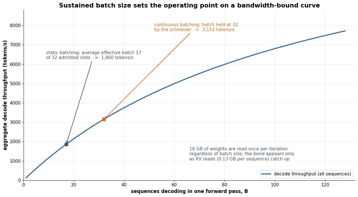

Line chart of aggregate decode throughput in tokens per second versus the number of sequences in the decode batch, from one to one hundred twenty-eight, for an eight-billion-parameter fp16 model with a one-thousand-token context on a two-terabyte-per-second GPU. The curve rises steeply and then bends as KV cache reads grow, with two marked points: an average effective batch of seventeen for static batching at about eighteen hundred tokens per second, and a sustained batch of thirty-two for continuous batching at about thirty-two hundred tokens per second.

Figure 2: Decode throughput against sustained batch size for an 8B fp16 model with 1K-token contexts on a 2 TB/s GPU. The curve is bandwidth-bound everywhere in this range, so throughput rises almost linearly at small $B$ and bends only as KV reads start to rival the 16 GB weight read. Continuous batching does not move the curve; it moves the operating point, from the average effective batch a draining static group achieves to the memory-limited maximum.

Mathematical Formulation:
$U_{\mathrm{static}} = \frac{\sum_{i=1}^{B} L_i}{B \, L_{\max}}$
$b_{\mathrm{kv}} = 2 \, n_l \, h_{kv} \, d_h \, s$
$t_{\mathrm{step}}(B) \approx \frac{2P + B \bar{L} b_{\mathrm{kv}}}{\mathrm{BW}}$
$\lambda(B) = B \, / \, t_{\mathrm{step}}(B)$
$B_{\max} = M_{\mathrm{free}} \, / \, (\bar{L} \, b_{\mathrm{kv}})$

Where:

$U_{\mathrm{static}}$ is the fraction of batch slot-iterations that produce a token under static batching, with $L_i$ the output length of request $i$ and $L_{\max} = \max_i L_i$ ; it is exactly 1 only when all lengths are equal.
$b_{\mathrm{kv}}$ is KV bytes per token, where $n_l$ is layers, $h_{kv}$ key/value heads (small under GQA), $d_h$ head dimension, $s$ bytes per element, and the leading 2 counts K and V.
$P$ is the parameter count, so $2P$ bytes is the fp16 weight read paid once per iteration regardless of $B$ , and $\mathrm{BW}$ is achievable HBM bandwidth.
$\bar{L}$ is the mean context length in the running batch and $B$ the number of sequences decoding in one forward pass.
$\lambda(B)$ is aggregate decode throughput in tokens per second; it is concave in $B$ because the KV term grows with $B$ while the weight term does not.
$M_{\mathrm{free}}$ is HBM left after weights and activations, so $B_{\max}$ is the admission ceiling the scheduler targets; the formula assumes $\bar{L}$ stays bounded, which it does not for sequences still growing.

Throughput At Two Operating Points (8B fp16, 1K context, 2 TB/s):
$\bar{L} \, b_{\mathrm{kv}} = 1024 \times 128\ \mathrm{KB} = 0.13\ \mathrm{GB}$
$t_{\mathrm{step}}(17) = 18.2 / 2000 = 9.1\ \mathrm{ms}$
$t_{\mathrm{step}}(32) = 20.2 / 2000 = 10.1\ \mathrm{ms}$
$\lambda(17) \approx 1870$
$\lambda(32) \approx 3170$

The byte totals are the 16 GB weight read plus $B \times 0.13$ GB of KV, divided by 2000 GB/s. Nearly doubling the sustained batch costs only 11% more time per step and yields 1.7x the tokens per second, which is the whole economic case for iteration-level scheduling: the extra sequences ride along in memory traffic that was already being paid.

Property	Static (request-level) batching	Continuous (iteration-level) batching	Continuous + chunked prefill
Scheduling unit	One whole generation loop per group	One forward pass	One forward pass with a token budget split across prefill and decode
Wait for a new arrival	Until the longest sequence in the current group finishes	One iteration, if KV blocks are free	One iteration, and its prefill is spread over several
Wasted compute	Pad tokens plus idle slots, growing with length variance	Near zero: ragged attention, no padding	Near zero, with better SM occupancy on decode-only steps
KV memory model	Contiguous buffer reserved for max length per slot	Paged blocks allocated on demand, freed on retirement	Same paged blocks, filled incrementally during prefill
Inter-token latency	Stable within a group, terrible queueing before it	Spikes whenever a long prompt is admitted	Bounded by the chunk size, at slightly higher TTFT
Dominant failure mode	Throughput collapse under heavy-tailed output lengths	KV exhaustion causing preemption and recompute thrash	Chunk size mistuned, trading TTFT against throughput

August 19, 2026

DL0132 LLM Serving Latency: TTFT and ITL

How do you measure and reduce Time to First Token (TTFT), Inter-Token Latency (ITL), and latency variance in a production LLM API such as a streaming chat endpoint served with vLLM?

Answer

TTFT is the wall-clock time from request arrival to the first streamed token and ITL is the gap between consecutive tokens after that, and they are separate metrics because they are produced by two phases with two different hardware bottlenecks. Prefill processes the whole prompt in one or a few forward passes and is compute-bound, so $T_{ttft}$ grows roughly linearly with prompt length; decode generates one token per forward pass and is memory-bandwidth-bound, so $T_{itl}$ is floored by the time to stream the weights and KV cache out of HBM. Measurement must happen at the streaming boundary and be reported as a distribution, namely p50, p95 and p99 merged from histograms and bucketed by input and output length, because a p99 computed over a mix of 200-token and 100k-token prompts is meaningless. Reduction is metric-specific: prefix caching and chunked prefill cut TTFT, FP8 quantization and speculative decoding cut ITL, and the variance work is almost entirely about removing things that can stall the decode loop, namely unchunked prefills, KV cache preemption, and queueing above roughly 70% utilization. The metric that actually decides capacity is goodput, the request rate you can sustain while both the TTFT and ITL SLOs hold at p99, not raw tokens per second.

(1) Two Phases, Two Bottlenecks: prefill is compute-bound and sets TTFT, decode is bandwidth-bound and sets ITL, so a change that helps one often does nothing for the other.
(2) Measure Distributions, Not Means: record one TTFT scalar plus an ITL vector of length $N_{out} - 1$ per request, and merge t-digest or HDR histograms across replicas instead of averaging per-replica p99s.
(3) TTFT Is Mostly Queueing Under Load: split server-side spans into $T_{queue}$ and $T_{prefill}$ , because past about 70% utilization the queue term dominates and no kernel optimization will help.
(4) The ITL Tail Is Interference, Not Steady State: p50 ITL reflects the decode step, while p99 ITL reflects the longest single stall, typically a colliding prefill or a preempted request being recomputed.
(5) Knobs Map To Metrics: prefix caching, chunked prefill and admission control for TTFT; quantization, GQA and speculative decoding for ITL; batch caps and prefill-decode disaggregation for variance.
(6) Optimize Goodput: report the sustained rate under both SLOs simultaneously, since raising batch size always trades TTFT and ITL tails for throughput.

Two timeline rows for one decoding request. In the baseline row, queue and prefill produce the first token, then four decode steps are interrupted by one wide unchunked prefill block that stalls the decode loop, creating a large inter-token gap. In the chunked-prefill row, the same prefill is split into six narrow chunks interleaved with decode steps, so every inter-token gap stays small.

Figure 1: TTFT is queue time plus prefill time; ITL is whatever happens between two decode steps of the same request. A single unchunked prefill scheduled into the shared loop stalls every decoding stream at once, which is the dominant source of p99 ITL. Splitting it into token-budgeted chunks bounds the worst stall to one chunk, at a small throughput cost from re-reading weights more often.

Instrument at the streaming boundary rather than inside the model: timestamp request arrival, the first SSE data event, and every subsequent event, then derive TTFT and the ITL vector client-side while the server emits its own queue, prefill and decode spans for the same request ID. The two views disagree in informative ways, because proxy buffering (an nginx deployment with proxy_buffering on) and a slow client event loop both inflate measured ITL with zero GPU involvement. For load testing, drive the endpoint with realistic input and output length distributions, since synthetic fixed-length prompts hide exactly the length-mixing effects that create the real tail; the vLLM benchmark_serving script and NVIDIA GenAI-Perf both report TTFT and ITL percentiles at a fixed request rate, which is the right shape of experiment. The variance checklist beyond scheduling is mundane but produces most of the surprises in practice: KV cache preemption and recompute when cache headroom runs out, ITL growing with batch size as decode drifts toward compute-bound, CUDA graph misses on uncaptured batch shapes, tensor-parallel all-reduce jitter, autoscaler cold starts that load tens of gigabytes of weights, and speculative decoding turning ITL bimodal because accepted-draft steps emit several tokens at once while rejected steps emit one.

Mathematical Formulation:
$T_{e2e} = T_{ttft} + (N_{out} - 1)\, \overline{T_{itl}}$
$T_{ttft} = T_{queue} + T_{prefill}$
$T_{prefill} \approx \frac{2 N_{in} P}{C_{eff}}$
$T_{itl} \geq \frac{B_{w} + B_{kv}}{BW}$
$T_{itl}^{spec} \approx \frac{T_{step}}{\mathbb{E}[n_{acc}]}$
$G = \lambda \cdot \Pr(T_{ttft} \leq S_{t},\ T_{itl} \leq S_{i})$

Where:

$T_{e2e}$ is end-to-end request latency, $T_{ttft}$ the time to first token, and $\overline{T_{itl}}$ the mean inter-token latency (its reciprocal is the perceived tokens per second of one stream).
$T_{queue}$ is scheduler wait time and $T_{prefill}$ the prompt forward pass; separating them is the single most useful piece of instrumentation, because they need opposite fixes.
$N_{in}$ and $N_{out}$ are prompt and completion token counts, $P$ the parameter count, and $C_{eff}$ the achieved (not peak) FLOP/s; the factor 2 counts one multiply and one add per parameter per token.
$B_{w}$ and $B_{kv}$ are the weight and KV cache bytes read per decode step and $BW$ is per-device HBM bandwidth, so this inequality is the bandwidth floor on ITL that no batching removes.
$T_{step}$ is one verification forward pass and $\mathbb{E}[n_{acc}] \geq 1$ the expected accepted tokens per step under speculative decoding, which divides effective ITL but widens its distribution.
$\lambda$ is offered request rate, $S_{t}$ and $S_{i}$ the TTFT and ITL SLO thresholds, and $G$ the resulting goodput, the only capacity number worth putting in a dashboard.

Plugging in real hardware makes the two bottlenecks concrete. A 70B model in BF16 needs roughly 140 GB of weights, so on eight H100s with tensor parallelism each device reads about 17.5 GB per decode step against roughly 3.35 TB/s of HBM, giving a floor near 5 ms per token before all-reduce and KV reads, which is why a single stream tops out around 100 to 150 tokens per second in practice. The same eight GPUs prefill a 2048-token prompt in about $2 \cdot 2048 \cdot 70$ B FLOPs, roughly 287 TFLOPs, which at an achieved 3.2 PFLOP/s is about 90 ms; a 32k-token prompt is 16 times that, which is exactly why long-context traffic destroys a shared TTFT SLO unless prefixes are cached or prefill is disaggregated. Note that FP8 weights halve $B_w$ and therefore the ITL floor, but barely move TTFT, while prefix caching can cut TTFT by an order of magnitude on a 1500-token shared system prompt and does nothing for ITL.

Two line charts against offered request rate. Left panel shows p50 and p99 TTFT in milliseconds rising sharply near capacity with a dotted 1500 ms SLO line and a vertical marker at the crossing rate. Right panel shows p50 and p99 inter-token latency in milliseconds with a dotted 80 ms SLO line crossed at a lower request rate, marking the binding constraint.

Figure 2: Both p50 curves stay flat while the p99 curves bend upward, because queueing and interference hit the tail first. Here the ITL SLO is crossed at a lower rate than the TTFT SLO, so goodput is ITL-bound and the correct response is to cap batch size or disaggregate, not to add prefill compute.

Technique	Metric it moves	What it costs
Prefix / KV cache reuse	TTFT p50 and p99 on shared system prompts, often 5x to 10x	HBM held by cached blocks, eviction policy tuning, cross-tenant isolation concerns
Chunked prefill	ITL p99 (bounds the worst decode stall to one chunk)	Slightly higher TTFT and a few percent lower throughput from repeated weight reads
Prefill-decode disaggregation	Both tails, by giving each phase its own pool and SLO	A KV cache transfer per request, duplicated weights, needs fast interconnect
Speculative decoding	ITL p50, roughly divided by accepted tokens per step	Bimodal ITL, wasted FLOPs on rejection, gains shrink at large batch sizes
FP8 or INT4 weight quantization	ITL floor, by halving or quartering bytes read per step	Accuracy regression that must be evaluated per task, calibration pipeline
Batch cap plus admission control	Latency variance, by refusing to accept work that will miss the SLO	Lower throughput and visible queueing or 429s, so it needs a priority policy

August 17, 2026

DL0091 Quantization Formats

What is quantization (FP16/BF16/INT8/INT4), and how does it affect model memory and accuracy?

Answer

Quantization stores weights, activations, or KV-cache entries in a numeric format with fewer bits than the FP32 values the model was defined in, trading numerical resolution for memory and bandwidth. Memory falls almost exactly linearly in bit width: a 70B-parameter model occupies 280 GB in FP32, 140 GB in FP16 or BF16, 70 GB in INT8, and roughly 37 GB in 4-bit with group scales. The two 16-bit floating formats differ only in how they split the 16 bits: FP16 spends 5 bits on the exponent and 10 on the mantissa (max magnitude 65,504, so gradients can overflow without loss scaling), while BF16 keeps FP32’s 8 exponent bits and truncates the mantissa to 7, giving the full $10^{38}$ dynamic range at coarser resolution. Below 16 bits the formats become integers plus a scale, so a real number is recovered as $\hat{w} = s(w_q - z)$ , and quality now depends on how finely those scales are estimated. In practice INT8 weights are essentially free in accuracy with per-channel scales, INT4 weight-only costs a few tenths of a perplexity point on a 70B model with a good calibration method, and quantizing activations is the hard part because transformer activations contain a handful of channels with magnitudes 20x to 100x the median.

(1) Exponent Versus Mantissa: FP16 and BF16 use the same 16 bits, but BF16’s 8 exponent bits buy dynamic range at the cost of precision, which is why BF16 is the default training format on modern accelerators and needs no loss scaling.
(2) Memory Is Linear In Bits: parameter memory is $N b / 8$ bytes, so each halving of the bit width halves the checkpoint, the resident weights, and the bytes moved per token.
(3) Integers Need A Scale And A Granularity: per-tensor scaling is cheapest, per-channel is the practical minimum for weights, and group-wise (typically 128 weights per scale) is what makes 4 bits usable.
(4) Weight-Only Helps Because Decode Is Bandwidth-Bound: single-stream generation reads every weight per token, so 4-bit weights cut latency even when the matmul itself runs in FP16 after dequantization.
(5) Error Concentrates In Outliers: a single extreme value stretches the scale and destroys resolution for every other value in the group, which is why outlier handling matters more than the nominal bit count.

Bit-field diagram comparing FP32, FP16, BF16, FP8 E4M3, INT8 and INT4: each format is drawn as a proportional bar split into sign, exponent and mantissa fields, with dynamic-range notes on the right

Figure 1: Bit budgets drawn to scale. BF16 keeps FP32’s 8 exponent bits and pays with 7 mantissa bits, FP16 does the reverse, and the sub-8-bit formats drop the exponent entirely in favour of an external scale factor.

An integer format is defined by an affine map from the real line onto $2^b$ evenly spaced levels. Symmetric quantization fixes the zero-point at $z = 0$ and is the standard choice for weights, whose distribution is roughly zero-centred; asymmetric quantization keeps a learned $z$ and suits post-ReLU or post-GELU activations that sit mostly on one side of zero. The granularity of $s$ is the real design knob: one scale per tensor stores nothing extra but is destroyed by a single outlier channel, whereas one scale per group of $g = 128$ weights adds a 16-bit scale and a 16-bit zero-point per group, which raises an INT4 tensor from 4.0 to 4.25 effective bits. Calibration methods such as GPTQ and AWQ then choose the rounding of each weight to minimise the error of the layer output on a small calibration set rather than the error of the weight itself, which is what closes most of the remaining gap at 4 bits.

Mathematical Formulation:
$\hat{w} = s (w_q - z)$
$w_q = \mathrm{clip}(\mathrm{round}(w/s) + z,\ 0,\ 2^b - 1)$
$s = \frac{\max(w) - \min(w)}{2^b - 1}$
$b_{eff} = b + \frac{32}{g}$
$M = \frac{N \, b_{eff}}{8}$

Where:

$\hat{w}$ is the dequantized value actually used in the matmul, and $w$ is the original FP32 or BF16 weight.
$w_q$ is the stored integer code, clipped into $\{0,\ldots,2^b-1\}$ ; values outside the calibrated range are saturated rather than wrapped.
$s$ is the scale (step size) and $z$ the zero-point; symmetric quantization sets $z = 0$ and uses $s = \max|w| / (2^{b-1} - 1)$ .
$b$ is the nominal bit width and $g$ the group size, the number of weights sharing one $(s, z)$ pair stored in FP16, hence the $32/g$ overhead.
$b_{eff}$ is the effective bits per weight; with $b = 4$ and $g = 128$ this gives $b_{eff} = 4.25$ .
$N$ is the parameter count and $M$ the weight memory in bytes; for $N = 7 \times 10^{10}$ this is about 37 GB. Required condition: $s > 0$ must be computed from calibration data before any activation quantization is applied.

Bar chart of weight memory in gigabytes for a 70 billion parameter model: 280 GB in FP32, 140 GB in FP16 or BF16, 70 GB in INT8 and 37 GB in INT4 with group size 128, with a dashed line marking the 80 GB capacity of one GPU

Figure 2: Weight memory for a 70B model. Only the 4-bit variant fits one 80 GB GPU with room left for the KV cache, and because decoding is memory-bandwidth bound the same reduction shows up directly in tokens per second.

Property	FP16	BF16	INT8	INT4 (g=128)
Layout	1 sign, 5 exponent, 10 mantissa	1 sign, 8 exponent, 7 mantissa	8-bit integer plus a per-channel FP16 scale	4-bit integer plus a scale per 128 weights
Dynamic range	Max 65,504; underflows below 6e-5	Same as FP32, about 3.4e38	256 levels inside the calibrated range	16 levels per group; clipping is the main risk
70B weights	140 GB	140 GB	70 GB	About 37 GB at 4.25 effective bits
Typical role	Inference, and training with loss scaling	Default training and master-weight format	W8A8 serving at high batch, compute-bound prefill	Weight-only decode on capacity-limited GPUs
Accuracy cost	None measurable for inference	None measurable; the lost mantissa bits rarely matter	Under 1% with per-channel scales and outlier handling	A few tenths of perplexity on 70B, clearly worse below 7B
Hardware support	Tensor cores on every recent GPU	Ampere onward, plus TPUs	Roughly 2x the FP16 matmul throughput	No native 4-bit matmul on most GPUs; kernels dequantize in registers

August 16, 2026

DL0090 Post-Training vs Quantization-Aware Training

What is the difference between post-training quantization and quantization-aware training, and how would you choose between them when shipping a model to an on-device NPU?

Answer

Post-training quantization (PTQ) takes a finished float checkpoint and converts it to low precision after the fact: a few hundred unlabeled samples are pushed through the network so the tool can observe activation ranges, pick a scale and zero point per tensor or per channel, and round the weights. No labels, no loss, no backward pass, and typically minutes to a couple of hours on a single GPU. Quantization-aware training (QAT) instead inserts fake-quantization nodes into the graph and continues training, so every forward pass sees rounded values while gradients flow through the non-differentiable rounding step via the straight-through estimator (STE). The one-line distinction worth memorizing: PTQ fits the quantizer to fixed weights, while QAT moves the weights to fit the quantizer. At INT8 on a well-behaved network the two land within a few tenths of a point of each other, so PTQ wins on cost; at 4 bits and below, or on outlier-heavy and depthwise-separable models, PTQ falls off a cliff and QAT recovers most of the loss.

(1) Where It Happens: PTQ is a post-processing step on a frozen checkpoint; QAT is a fine-tuning stage that must run inside your training pipeline with the original data loader and loss.
(2) What Data It Needs: PTQ needs only a small calibration set (roughly 128 to 1024 unlabeled samples) that is representative of deployment traffic; QAT needs labeled data, or at least a teacher model for distillation.
(3) The STE Trick: rounding has zero gradient almost everywhere, so QAT pretends the quantizer is the identity inside the clipping range and passes the gradient straight through, which is what lets weights drift toward values that round well.
(4) Where PTQ Breaks: per-tensor scales collapse when channel ranges differ by orders of magnitude (depthwise convolutions), when activations carry massive outliers (transformer residual streams), or when the bit width drops to 4 or fewer.
(5) Decision Rule: always try PTQ first because it is cheap and reversible; escalate to QAT only when a measured accuracy gap survives per-channel scales, better range selection, and bias correction.

Mechanically, a fake-quant node applies quantize → dequantize in the forward pass, so tensors stay in float during QAT but carry exactly the values the integer kernel will produce at inference. That means QAT does not speed up training; it slows it down by 20 to 40 percent while simulating the deployment numerics. The payoff is that the optimizer sees the rounding error as part of the loss surface and settles into flatter minima where a few least significant bits do not matter. PTQ has no such feedback: whatever error the rounding introduces is simply propagated forward, which is why its failure mode is a sudden collapse rather than a graceful slide.

Two horizontal pipelines. Top row, post-training quantization: trained FP32 checkpoint, calibration pass on 128 to 1024 unlabeled samples, fit scale and zero point, export INT model. Bottom row, quantization-aware training: trained FP32 checkpoint, insert fake-quant nodes, fine-tune with labels and STE gradients, fold scales and export INT model.

Figure 1: The same checkpoint, two routes to integer inference. PTQ adds one forward-only calibration pass; QAT adds a full fine-tuning loop whose gradients reach the weights through the straight-through estimator.

Mathematical Formulation:
$s = \frac{x_{max} - x_{min}}{2^{b} - 1}$
$q = \mathrm{clip}(\lfloor x/s \rceil + z, 0, 2^{b} - 1)$
$\hat{x} = s\,(q - z)$
$\frac{\partial \mathcal{L}}{\partial x} \approx \frac{\partial \mathcal{L}}{\partial \hat{x}} \cdot \mathbf{1}[x_{min} \leq x \leq x_{max}]$

Where:

$\hat{x}$ is the dequantized value the network actually computes with, and $x$ is the original float weight or activation.
$s$ is the scale and $z$ the zero point (the integer that maps to exactly 0.0); $q$ is the stored integer code.
$b$ is the bit width, so $b = 8$ gives 256 levels and $b = 4$ only 16; $x_{min}, x_{max}$ are the calibrated clipping bounds, chosen per channel for weights and per tensor or per token for activations.
$\lfloor \cdot \rceil$ is round-to-nearest and $\mathrm{clip}$ saturates values outside the representable range; both are the source of the error being managed.
The last line is the straight-through estimator: the indicator $\mathbf{1}[\cdot]$ passes the gradient unchanged inside the clipping range and zeroes it outside, which is the only reason QAT can backpropagate through rounding.
PTQ solves for $s, z$ with $x$ held fixed; QAT keeps the whole chain in the graph and updates $x$ (and, with learned-step methods, $s$ itself).

Line chart of top-1 accuracy versus bit width from INT8 down to INT2. PTQ tracks the FP32 baseline at INT8 and INT6 but drops to 68 at INT4, 41 at INT3 and 6 at INT2, while QAT stays at 74.5 at INT4, 71 at INT3 and 62 at INT2.

Figure 2: Illustrative accuracy versus bit width. The two methods are indistinguishable at INT8, which is why PTQ dominates production INT8 pipelines; the gap opens abruptly at 4 bits and below, where the rounding error stops behaving like small additive noise.

Dimension	Post-Training Quantization	Quantization-Aware Training
Data needed	128 to 1024 unlabeled calibration samples	Labeled training data or a teacher for distillation
Compute	Minutes to hours, one GPU, forward passes only	Hours to days, often multi-GPU, full training loop
Pipeline access	Works on a vendor or third-party checkpoint	Requires the original recipe, loss and hyperparameters
Typical INT8 result	Within roughly 0.5 points of FP32 with per-channel weights	Essentially lossless, rarely worth the cost
Typical INT4 result	Large drop unless advanced methods (GPTQ, AWQ) are used	Recovers most of the gap, the standard choice below 4 bits
Iteration speed	Cheap to sweep many bit widths and granularities	Each configuration is a separate training run

August 15, 2026

ML0086 Drift Detection in Production

How would you detect data drift in a deployed machine learning model?

Answer

You monitor in layers, because no single statistic sees everything. Layer one watches the inputs: per-feature distribution statistics (PSI, KS distance) of live traffic against the training baseline. Layer two watches the outputs: the prediction distribution and confidence profile, which catch label shift and model-side anomalies. Layer three estimates or measures performance: delayed ground truth when it arrives, and label-free estimators like NannyML’s CBPE in the gap. Each layer has thresholds with alerting, and alerts route to a decision: investigate the pipeline, retrain, or roll back. The whole pattern is standardized in AWS SageMaker Model Monitor: a baseline job computes statistics and constraints from training data, scheduled jobs compare live captures, and violations fire CloudWatch alarms.

(1) Baseline vs Window: freeze reference statistics from the training distribution, then compute drift metrics over sliding or scheduled production windows; the metric is a distance between two empirical distributions, not a model property.
(2) What Each Layer Sees: input stats see covariate shift, output stats see label shift and confidence collapse, and only ground truth (or calibrated estimation) sees concept drift; NannyML’s CBPE handles covariate shift but explicitly not concept drift.
(3) Production Pattern (AWS): Model Monitor’s built-in container (Deequ on Spark) emits statistics.json and constraints.json from a baseline, then scheduled monitoring jobs check distribution distance (linf_simple / two-sample KS via linf_robust, LInfinity or ChiSquared for categoricals) and write violation reports that drive alarms. AWS has announced that Model Monitor closes to new customers on 30 July 2026, with existing customers unaffected, but this baseline/constraints/violations design remains the reference pattern.

PSI over weekly production windows: values hover low for months, cross the moderate threshold, then breach the significant threshold where an alarm marker fires

Figure 1: A drift monitor in action: per-window PSI against the training baseline crosses the moderate band (0.1) and then the significant band (0.25), which is where alerting and retraining triggers fire.

Design details separate a working monitor from alert fatigue. Thresholds must account for sample size (small windows inflate every distance metric), per-feature tests need multiplicity control or aggregation, and the window length trades detection latency against statistical power. When labels are delayed, record them when they land and backfill realized metrics so you can audit how well the label-free estimators tracked reality. Finally, every alert needs a playbook: distinguish a broken upstream pipeline (schema violations, sudden null spikes) from genuine distribution drift, because the fix for the former is a data engineer, not a retraining job.

Monitoring stack flow: live traffic feeds input statistics checks and output confidence checks, delayed labels feed realized metrics, all signals join a decision block that routes to investigate, retrain, or roll back

Figure 2: The layered monitoring stack: input-distribution checks, output/confidence checks, and delayed-label evaluation feed one decision layer that separates pipeline breakage from genuine drift and triggers the right response.

Mathematical Formulation:
$\mathrm{PSI} = \sum_{b=1}^{B} (a_b - e_b)\,\ln\frac{a_b}{e_b}$
$D_{KS} = \max_x \, |F_{ref}(x) - F_{cur}(x)|$

Where:

$a_b$ and $e_b$ are the fractions of the current (actual) and reference (expected) samples in bin $b$ ; rules of thumb: PSI above 0.1 indicates moderate drift, above 0.25 significant drift.
$F_{ref}, F_{cur}$ are the empirical CDFs of the baseline and current window; $D_{KS}$ is their maximum vertical gap (the statistic behind SageMaker’s linf distance checks).
Both are computed per feature per window and compared against thresholds tuned for window size and alert budget.

Layer	Signal	Catches	Blind To
Input Stats	PSI / KS per feature vs baseline	Covariate shift, schema breakage	Concept drift
Output Stats	Prediction mix, confidence histogram	Label shift, confidence collapse	Silent concept drift
Estimated Performance	CBPE from calibrated probabilities	Accuracy loss under covariate shift	Concept drift (by assumption)
Delayed Ground Truth	Realized metrics when labels land	Everything, eventually	Nothing, but late

August 11, 2026