Tag: Tree

ML0087 AdaBoost vs Gradient Boosting

How does AdaBoost differ from gradient boosting, and why has gradient boosting become the production standard?

Answer

AdaBoost and gradient boosting are both sequential ensemble methods that add weak learners stage by stage, but they differ in what each new learner targets and how the loss is shaped. AdaBoost reweights training examples: misclassified samples get exponentially higher weights, and the next weak learner is fit on the reweighted data, then added with a stage weight set by the log-odds of its weighted error rate. Gradient boosting fits each new learner to the negative gradient of an arbitrary differentiable loss with respect to the current ensemble’s predictions, which generalizes to regression, ranking, and any custom loss. AdaBoost’s exponential loss is a special, fixed case; gradient boosting’s loss is a knob. In production, gradient boosting variants (XGBoost, LightGBM, CatBoost) dominate tabular ML, while AdaBoost is largely legacy, and scikit-learn even removed the SAMME.R variant in 2024.

(1) Reweighting vs Gradient Fitting: AdaBoost changes sample weights via the exponential loss and refits on the weighted distribution; gradient boosting fits each tree to pseudo-residuals, the negative gradient of whatever loss you choose.
(2) Fixed vs Arbitrary Loss: AdaBoost’s reweighting rule is tied to the exponential loss (SAMME for multi-class), so a different task needs a different algorithm (regression uses AdaBoost.R2); gradient boosting swaps in squared error, logistic loss, quantile loss, Huber, or a custom loss without changing the algorithm, covering regression, classification, and ranking.
(3) Production Dominance: gradient boosting frameworks (XGBoost, LightGBM, CatBoost) dominate tabular ML in production, while AdaBoost appears only in niche ensembles; scikit-learn removed SAMME.R in version 1.6 (deprecated one release earlier) because the algorithm was based on a preprint never published in its final form.

Side-by-side flow: AdaBoost panel shows sample weights increasing on misclassified points then refitting a stump; gradient boosting panel shows pseudo-residuals computed from the loss gradient then fitting a tree to those residuals

Figure 1: AdaBoost updates sample weights via the exponential loss and refits on the reweighted distribution, while gradient boosting computes pseudo-residuals as the negative gradient of an arbitrary loss and fits the next tree to those residuals.

The exponential loss also makes AdaBoost fragile in ways gradient boosting is not. Because misclassified samples receive exponentially growing weights, a single noisy label or outlier can dominate subsequent stages, pulling the ensemble toward the noise. Gradient boosting’s gradient-based approach spreads the influence of an outlier according to the loss derivative, and modern frameworks add regularization (shrinkage, tree depth limits, column subsampling, early stopping) that AdaBoost lacks natively. A 2024 NeurIPS paper proved that boosting can in principle optimize essentially any loss, without requiring convexity, differentiability, or even continuity, but this remains theoretical; in practice, gradient boosting’s differentiable-loss flexibility plus regularization is what made XGBoost, LightGBM, and CatBoost the de facto tabular standard.

Mathematical Formulation:
$w_i^{(m+1)} = \frac{w_i^{(m)} \exp\!\big(\alpha_m\, \mathbb{1}[y_i \neq h_m(x_i)]\big)}{Z_m}$
$F_m(x) = F_{m-1}(x) + \nu\, h_m(x)$
$r_{i,m} = -\left[\frac{\partial\, \ell(y_i, F)}{\partial\, F}\right]_{F = F_{m-1}}$

Where:

$w_i^{(m)}$ is the AdaBoost weight of example $i$ at stage $m$ , $\alpha_m = \tfrac{1}{2}\ln\frac{1 - \text{err}_m}{\text{err}_m}$ is the stage weight (half the log-odds of being correct), and $Z_m$ normalizes the weights so they sum to 1.
$F_m(x)$ is the gradient boosting ensemble after stage $m$ , $h_m$ is the tree fit to the pseudo-residuals, and $\nu$ is the learning rate (shrinkage).
$r_{i,m}$ is the pseudo-residual: the negative gradient of the chosen loss $\ell$ with respect to the current prediction. For squared loss this reduces to the ordinary residual $y_i - F_{m-1}(x_i)$ ; for logistic loss it is $y_i - \sigma(F_{m-1}(x_i))$ .

Aspect	AdaBoost	Gradient Boosting
What Each Stage Targets	Reweighted samples (exponential loss upweights errors)	Pseudo-residuals (negative gradient of arbitrary loss)
Loss Function	Fixed: exponential (SAMME for multi-class)	Arbitrary differentiable: squared, logistic, Huber, quantile
Task Coverage	Classification; regression via separate AdaBoost.R2	Classification, regression, ranking, survival
Noise Robustness	Fragile: exponential weights amplify outliers	Robust: regularization, shrinkage, robust losses
Production Status	Legacy; SAMME.R removed from scikit-learn 1.6 (2024)	Dominant: XGBoost, LightGBM, CatBoost

August 12, 2026

ML0082 XGBoost Improves Gradient Boosting

How does XGBoost improve upon the classical gradient-boosted decision tree algorithm?

Answer

XGBoost keeps the sequential additive recipe of classical gradient boosting but upgrades it on three axes. First, optimization: it fits each tree with a second-order Taylor approximation of the loss, using both gradients and Hessians, so leaf weights and split gains are Newton-style steps instead of plain gradient steps. Second, regularization: the objective explicitly penalizes the number of leaves and the squared leaf weights, which prunes weak splits analytically. Third, systems: sparsity-aware split finding, a weighted quantile sketch for approximate splits, and cache-aware block layouts let it scale to billions of examples. The result dominated competitions: 17 of the 29 winning solutions published on Kaggle’s blog in 2015 used XGBoost.

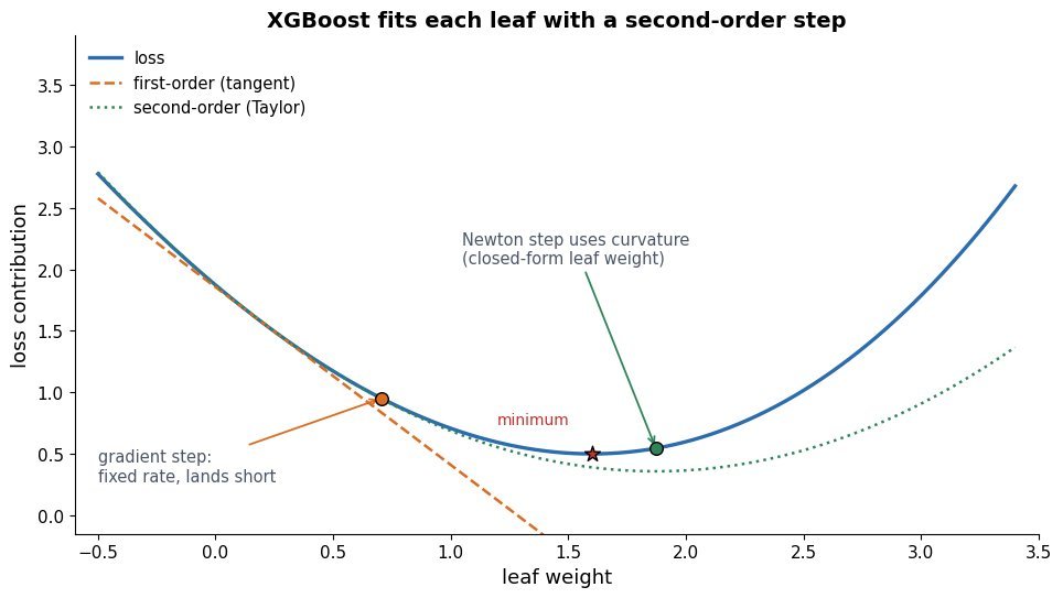
(1) Second-Order Optimization: gradients alone say which way is downhill; Hessians say how curved the surface is, so XGBoost computes closed-form optimal leaf weights and exact split gains per candidate split.
(2) Regularized Objective: the penalty on leaf count and weight magnitude means a split must beat an explicit complexity cost to survive, a built-in analogue of pruning that classical GBDT lacks.
(3) Systems Engineering: default directions for missing values, approximate split proposals from weighted quantiles, and out-of-core cache-aware blocks deliver the reported 10x-plus speedups that made it the industry default.

One-dimensional loss curve with a gradient-only step undershooting the minimum while a second-order Newton step, using curvature, lands near it

Figure 1: Why the Hessian helps: a first-order step moves along the tangent and misses the valley; a second-order step accounts for curvature (dashed parabola) and lands near the minimizer, which is what closed-form leaf weights do for every leaf.

The second-order view also explains where the regularization bites. Once you collect all examples routed to a leaf, the objective contribution of that leaf is a one-dimensional quadratic in its weight, whose closed-form minimizer shrinks toward zero as the penalty grows. Splits are scored by how much they reduce the total objective including the per-leaf cost, so a split that adds two leaves must overcome an explicit gamma toll twice. Classical GBDT instead fits trees to raw gradients and controls complexity only indirectly through depth caps and shrinkage.

Mathematical Formulation:
$\mathcal{L}^{(t)} \simeq \sum_{i=1}^{N} \left[ g_i f_t(x_i) + \frac{1}{2} h_i f_t^2(x_i) \right] + \Omega(f_t)$
$\Omega(f) = \gamma T + \frac{1}{2}\lambda \sum_{j=1}^{T} w_j^2$
$w_j^* = -\frac{G_j}{H_j + \lambda}$

Where:

$g_i$ and $h_i$ are the first and second derivatives of the per-example loss at the current prediction; $f_t$ is the new tree.
$\Omega(f)$ is the regularizer: $\gamma$ charges per leaf ( $T$ leaves) and $\lambda$ penalizes squared leaf weights $w_j$ .
$G_j, H_j$ are the sums of $g_i, h_i$ over the examples routed to leaf $j$ , and $w_j^*$ is the closed-form optimal leaf weight; larger $\lambda$ shrinks every leaf toward zero.

Aspect	Classical GBDT	XGBoost
Loss Information	First-order gradients (residuals)	Gradients + Hessians (second-order Taylor)
Regularization	Indirect: depth caps, shrinkage, subsampling	Explicit: gamma on leaf count, lambda on leaf weights
Split Finding	Exact scan or basic histograms	Weighted quantile sketch + sparsity-aware defaults
Scale	In-memory, single machine	Cache-aware blocks, out-of-core, distributed
Track Record	Strong but slow at scale	17 of 29 Kaggle 2015 winning solutions; every KDDCup 2015 top-10 team

August 11, 2026

ML0081 Gradient Boosting vs Random Forest

How do gradient-boosted decision trees work, and how do they differ from random forests?

Answer

Gradient boosting builds an additive ensemble sequentially: each new tree is fit to the negative gradient of the loss with respect to the current ensemble’s predictions (for squared error, the residuals), then added in with a small learning rate. The ensemble is a directed attack on bias; every stage shrinks whatever error remains. A random forest does the opposite: it grows many deep trees independently on bootstrap samples with random feature subsets and averages their votes, which attacks variance. So boosting uses shallow trees, a learning rate, and sequence, while bagging uses deep trees, randomness, and parallel averaging.

(1) Sequential Residual Fitting: tree m targets the current gradient (pseudo-residuals); with squared loss this is literally y minus the running prediction, and shrinkage keeps any single tree from dominating.
(2) Bias vs Variance: boosting reduces bias stage by stage but can chase noise if run long or deep; random forests reduce variance by decorrelating many overfit trees, but their bias is roughly that of one tree.
(3) Modern Refinement: Yandex showed classic gradient boosting leaks target information into its own gradients (prediction shift), and CatBoost’s ordered boosting fixes it by computing each example’s gradient from a model trained only on earlier examples in a random permutation.

Three panels: initial prediction is flat with large residuals; after adding tree one the curve follows the data and residuals shrink; after tree two the fit is close and residuals are small

Figure 1: Stage-wise fitting: each new tree targets the residuals (orange stems) left by the current ensemble, so the prediction curve (blue) bends toward the data a little at every stage.

Structurally, the two ensembles could not be more different. A random forest is embarrassingly parallel: tree one and tree one hundred do not know each other, so you can train them on separate machines and the average cancels their individual overfitting. Gradient boosting is an inherently sequential chain: tree one hundred is defined by the mistakes of the previous ninety-nine, which buys accuracy on structured tabular data but makes training serial and makes the model sensitive to label noise, because late-stage trees are explicitly trained to fit whatever is left, including the noise.

Side-by-side schematics: random forest trains deep trees in parallel on bootstrap samples and averages votes; gradient boosting trains shallow trees in a chain where each consumes the previous ensemble's residuals

Figure 2: Parallel averaging vs sequential correction: the forest’s trees are independent and deep, the boosted trees are shallow and chained through residuals, with a learning rate throttling each contribution.

Mathematical Formulation:
$F_m(x) = F_{m-1}(x) + \nu\, h_m(x)$
$r_{i,m} = -\left[\frac{\partial\, \ell(y_i, F(x_i))}{\partial\, F(x_i)}\right]_{F = F_{m-1}}$

Where:

$F_m$ is the ensemble after stage $m$ , $h_m$ the tree added at that stage, and $\nu$ the learning rate (shrinkage, typically 0.01-0.1).
$r_{i,m}$ is the pseudo-residual for example $i$ : the negative gradient of the loss $\ell$ with respect to the current prediction, i.e. the direction that most reduces the loss.
For squared loss, $r_{i,m} = y_i - F_{m-1}(x_i)$ , the ordinary residual; other losses (logistic, absolute) change what the trees are fit to.

Aspect	Random Forest	Gradient Boosting
Training	Independent trees, bootstrap samples, fully parallel	Sequential; each tree fits current pseudo-residuals
Tree Shape	Deep, low-bias, high-variance	Shallow (depth 3-8), high-bias learners
What It Reduces	Variance (averaging decorrelated trees)	Bias (stage-wise error correction)
Noise Robustness	Robust; noise averages out	Fragile; late trees chase label noise
Known Issue	Averaging cannot reduce base-tree bias	Target leakage in gradients; fixed by CatBoost ordered boosting

August 11, 2026

ML0080 Decision Tree Pruning

Why do decision trees need pruning, and how is it done?

Answer

An unconstrained decision tree grows until every leaf is pure, which on real data means it memorizes noise: training accuracy hits 100% while test accuracy sags. Pruning is the cure, and it comes in two forms. Pre-pruning stops growth early with rules like maximum depth, minimum samples per leaf, or minimum impurity decrease. Post-pruning grows the full tree first, then cuts back the branches whose complexity is not repaid by fit, using a validation-based criterion such as cost-complexity pruning. Post-pruning is usually stronger because a split that looks useless alone may unlock a highly valuable subtree below it; pre-pruning can never see that.

(1) Why Trees Overfit: depth adds one axis-aligned cut per level, so a deep tree carves the training set into tiny pure cells, which is high variance by construction.
(2) Pre- vs Post-Pruning: pre-pruning is cheap but myopic (it can miss XOR-style interactions); post-pruning explores the full tree and then removes only the provably weakest links.
(3) Production Default: scikit-learn implements minimal cost-complexity pruning via the ccp_alpha parameter: its documented example shows an unpruned tree at 100% train / 88% test accuracy, while sweeping the pruning path finds ccp_alpha near 0.015 maximizing test accuracy.

Train and test accuracy versus ccp_alpha: train accuracy falls monotonically, test accuracy rises to a peak near alpha 0.015 then falls, marking the bias-variance sweet spot

Figure 1: The pruning path: as ccp_alpha grows, more of the tree is cut, training accuracy declines, and test accuracy peaks where complexity is repaid by generalization (the sklearn example peaks near 0.015).

Cost-complexity pruning scores each subtree by its error plus a per-leaf penalty, so a branch survives only if it reduces impurity enough to pay for its leaves. Pruning proceeds weakest-link-first: at each step the node whose removal costs the least accuracy per leaf is collapsed, producing a nested sequence of subtrees indexed by alpha. You then pick alpha by cross-validation rather than by training-set performance, which is what makes the chosen tree a generalization-optimal member of the sequence.

Two trees side by side: a deep full tree with many leaves and low purity, and its pruned version where dashed subtrees were collapsed into single leaves

Figure 2: Post-pruning in action: the full tree (left) contains branches fitted to noise; the dashed subtrees are the weakest links, and the pruned tree (right) collapses them into leaves.

Mathematical Formulation:
$R_{\alpha}(T) = R(T) + \alpha\,|\widetilde{T}|$
$\alpha_{eff}(t) = \frac{R(t) - R(T_t)}{|T_t| - 1}$

Where:

$R(T)$ is the total (sample-weighted) impurity of the leaves of tree $T$ , and $|\widetilde{T}|$ is its number of terminal nodes.
$\alpha$ is the complexity parameter (ccp_alpha in scikit-learn); larger alpha prunes more aggressively.
$\alpha_{eff}(t)$ is the effective alpha of node $t$ : the penalty value at which keeping its branch $T_t$ costs exactly as much as collapsing it, so the node with the smallest value is pruned first.

Aspect	Pre-Pruning (Early Stop)	Post-Pruning (Grow Then Cut)
Knobs	max_depth, min_samples_leaf, min_impurity_decrease	ccp_alpha chosen from cost_complexity_pruning_path by CV
Failure Mode	Myopic: stops before a weak-looking split that enables a strong subtree	Costs a full grow pass plus a validation sweep
Typical Accuracy	Good, knob-sensitive	Usually better; principled weakest-link order
When Used	Massive data, streaming, latency-critical fits	Default for single interpretable trees

August 11, 2026

ML0065 Random Forest III
How to choose the number of features in a random forest?
Answer
Select the number of features considered at each split (the $m$ , or max_features) by starting from the default heuristics, then tuning with cross-validation or out-of-bag (OOB) error to find the best value for your specific dataset. The choice trades bias against variance and accuracy against training cost.
(1) Default Heuristics: Classification: $m = \sqrt{p}$ ; regression: $m = p/3$ ; solid starting points.
(2) Bias-Variance Trade-Off: Smaller $m$ adds randomness: less correlated trees (lower variance) but potentially higher bias; larger $m$ strengthens each tree (lower bias) but correlates their errors (higher variance).
(3) Systematic Search: Grid or randomized search over a range of values with cross-validation is the most robust method; OOB error offers a validation-free alternative unique to bagged models.

Figure 1: CV accuracy across max_features on a 30-feature dataset: accuracy is poor when m is tiny (trees too weak), then plateaus with a noisy peak at m = 15; the $\sqrt{p} \approx 5.5$ heuristic lands inside the good region, and CV refinement picks the best value on the plateau.
Mathematical Formulation:
$m = \sqrt{p} \quad \text{(classification)}$
$m = \frac{p}{3} \quad \text{(regression)}$
Where:
$p$ is the total number of features in the dataset.
$m$ is the number of features randomly drawn and considered at each split (max_features in most libraries).
These are heuristics, not optima; cross-validation or OOB error refines them per dataset.
Login to view more content
July 19, 2025
ML0064 Random Forest II
Please explain the benefits and drawbacks of random forest.
Answer
Random forest is a powerful ensemble method that reduces overfitting and improves predictive accuracy by combining many decision trees. The trade-off: it sacrifices interpretability and computational efficiency, and it may require careful tuning on large, imbalanced, or sparse datasets.
(1) Benefit: Reduces Overfitting: Aggregating many trees lowers variance.
(2) Benefit: Robust: Less sensitive to noise and outliers; handles high-dimensional data well.
(3) Benefit: Feature Importance: Built-in estimates identify influential variables; bagging improves generalization.
(4) Drawback: Cost: Hard to interpret compared to a single tree; slower to train and predict; large forests consume significant memory.
(5) Drawback: Data Traps: Class imbalance can bias predictions, and very sparse data can make it underperform other algorithms.

Figure 1: The imbalance trap: on 96/4 skewed data the random forest’s regions bend toward the majority class and its minority-class F1 (0.73) loses even to a class-weighted logistic regression (0.76): a strong default is not automatically strong everywhere.
Mathematical Formulation:
$\mathrm{Var}\big(\bar{T}(x)\big) = \rho \, \sigma^2 + \frac{1 - \rho}{B} \, \sigma^2$
Where:
$\bar{T}(x)$ is the forest’s averaged prediction over $B$ trees, each with individual variance $\sigma^2$ .
$\rho$ is the pairwise correlation between trees: this is what bagging and random feature subsets try to shrink.
As $B \to \infty$ the second term vanishes but the $\rho\sigma^2$ floor remains: correlation, not tree count, is the limiting factor.
Login to view more content
July 8, 2025
ML0063 Random Forest
How does the random forest algorithm operate? Please outline its key steps.
Answer
Random Forest builds an ensemble of decision trees, each trained on a bootstrapped sample of the data with a random feature subset considered at each split. This combination reduces variance, combats overfitting, and improves predictive accuracy; the final output aggregates all trees’ predictions: majority vote for classification, averaging for regression.
(1) Bootstrap Sampling: Create multiple subsets of the training data by sampling with replacement (bootstrap samples).
(2) Grow Decision Trees: Train an unpruned decision tree on each bootstrap sample.
(3) Random Feature Selection: At every split in every tree, consider only a random subset of features; this increases diversity between trees.
(4) Aggregate: Classification: each tree votes for a class and the majority wins; regression: the tree outputs are averaged.

Figure 1: Three trees, three different jagged boundaries: each overfits its own bootstrap sample in its own way. The ensemble’s boundary (bottom right) averages the votes and lands smoother and closer to the true structure: the trees’ individual errors cancel.
Mathematical Formulation:
$\hat{y} = \mathrm{mode}\big\{ T_b(x) \big\},\quad b = 1, \ldots, B$
$\hat{y} = \frac{1}{B} \sum_{b=1}^{B} T_b(x)$
Where:
$T_b(x)$ is the prediction of the $b$ -th tree for input $x$ .
$B$ is the total number of trees in the forest.
First line: classification by majority vote (mode); second line: regression by averaging.

Figure 2: The full pipeline: B bootstrap replicas of the training set feed B independently grown trees (each with random feature subsets at its splits), and a majority-vote / averaging box fuses their outputs into one robust prediction.
Login to view more content
July 4, 2025
ML0062 Decision Tree
Please explain how a decision tree works.
Answer
A decision tree partitions the input space into regions by recursively splitting on the feature that best separates the target variable. Each split aims to improve the “purity” of the resulting subsets, measured by criteria such as Gini impurity or entropy. Predictions follow the sequence of splits down to a leaf, returning the most common class (classification) or the average target (regression).
(1) Structure: A tree of nodes: internal nodes test a feature, branches represent the outcomes, leaves give predictions.
(2) Splitting Criterion: Choose the best feature and threshold by maximizing purity: information gain (entropy), Gini impurity, or variance reduction for regression.
(3) Recursive Growth: Starting at the root, split the data, then recurse on each subset until stopping criteria are met (max depth, min samples, or pure leaves).
(4) Prediction: A new sample travels from root to leaf following the feature tests; the leaf’s label or value is returned.

Figure 1: A decision tree from two viewpoints: on the left, the axis-aligned rectangular regions it carves into the feature space; on the right, the tree itself: each node shows its test, impurity, and class counts, and each leaf is a final answer.
Mathematical Formulation:
$\mathrm{Gini}(t) = 1 - \sum_{k=1}^{K} p_k^2$
$\mathrm{Entropy}(t) = -\sum_{k=1}^{K} p_k \log_2(p_k)$
$\mathrm{Information\ Gain} = \mathrm{Entropy}(\mathrm{Parent}) - \sum_{i} \frac{N_i}{N} \, \mathrm{Entropy}(\mathrm{Child}_i)$
Where:
$t$ is a tree node; $K$ the number of classes; $p_k$ the proportion of class $k$ samples in node $t$ .
Gini = 0 means the node is pure (one class only) and grows with mixing; entropy = 0 at perfect purity and is maximal when classes are uniformly mixed.
In the gain formula, $N$ is the parent’s sample count and $N_i$ child $i$ ‘s: the split chosen is the one maximizing this weighted impurity drop.

Figure 2: The two classification criteria compared for a binary node: both peak at $p = 0.5$ (maximally mixed) and vanish at pure nodes; they nearly always rank candidate splits in the same order, which is why Gini (no logarithms) is the common default.
Login to view more content
June 30, 2025