Category: Hard

  • ML0088 SVM Scaling

    Why do SVMs scale poorly to very large datasets, and what can you do about it when you need to classify millions of samples?

    Answer

    The bottleneck is the kernel matrix. A kernel SVM solves a quadratic program whose dual involves an n \times n Gram matrix of pairwise kernel evaluations, which costs O(n^2) storage and between O(n^2) and O(n^3) time depending on the solver and regularization. Beyond tens of thousands of samples the full matrix no longer fits in memory, and the QP solver’s iteration count grows with the number of support vectors, which itself scales roughly linearly with n. Scikit-learn’s documentation states this explicitly: SVC “scales at least quadratically with the number of samples and may be impractical beyond tens of thousands of samples,” and recommends LinearSVC or SGDClassifier for large datasets. The production answer is to either drop the kernel (linear SVM), approximate it (Nyström, Random Fourier Features), or accelerate the computation on GPU (NVIDIA RAPIDS cuML).

    (1) Kernel Matrix Bottleneck: the dual QP requires the full n \times n kernel matrix in memory; at 1 million samples this is 8 TB in float64, and the solver time is superlinear in n.
    (2) Support Vector Growth: the number of support vectors grows roughly linearly with training size, so inference cost also grows with n, unlike a fixed-size linear model.
    (3) Production Solutions: scikit-learn recommends LinearSVC (liblinear, scales to millions) or kernel approximation via Nystroem transformer; RAPIDS cuML provides GPU acceleration for SVC and SVR; EigenPro 3.0 (ICML 2023) decoupled model size from data size, training on 5 million samples with 1 million centers.

    Line chart of relative training time versus training samples from 1K to 100K: kernel SVC curves upward quadratically, LinearSVC and Nystrom plus linear solver both rise linearly, with an annotation that kernel SVM becomes impractical beyond about 50K samples

    Figure 1: Training time versus dataset size: kernel SVM grows as O(n^2) to O(n^3) because of the full Gram matrix and QP solver, while linear SVM (LinearSVC) and Nyström-approximated kernel SVM both scale near-linearly with a larger constant for the approximation.

    The practical toolkit has four tiers. First, if a linear boundary is acceptable, use LinearSVC (liblinear) or SGDClassifier with hinge loss, both of which scale to millions of samples and features because they never form a kernel matrix. Second, if you need nonlinearity, approximate the kernel map: Nyström approximation samples m landmark points (m much less than n) and replaces the n-by-n matrix with a rank-m factorization, and Random Fourier Features (RFF) map data into an explicit finite-dimensional space where a linear solver applies; ICML 2024 showed Quasi-Monte Carlo features improve RFF’s error from O(1/sqrt(M)) to O(1/M). Third, GPU-accelerate: RAPIDS cuML provides zero-code-change GPU dispatch for SVC and SVR. Fourth, for true kernel-method scale, EigenPro 3.0 (ICML 2023) uses preconditioned SGD to train kernel models with 1 million centers on 5 million samples, decoupling model size from data size for the first time.

    Decision tree starting from a large dataset above 100K samples: if linearly separable use LinearSVC or SGDClassifier; if not, ask whether a GPU is available, where no leads to Nystrom or Random Fourier Features with a linear solver and yes leads to RAPIDS cuML or EigenPro 3.0

    Figure 2: A practical decision flow: linearly separable data uses LinearSVC or SGDClassifier; if the boundary must be nonlinear, CPU-only setups use Nyström or Random Fourier Features with a linear solver, while GPU hardware unlocks RAPIDS cuML or EigenPro 3.0’s preconditioned SGD.

    Mathematical Formulation:
    \min_{\alpha} \;\frac{1}{2}\alpha^\top Q\,\alpha - \mathbf{1}^\top \alpha
    \text{s.t.}\quad y^\top \alpha = 0,\quad 0 \leq \alpha_i \leq C
    Q_{ij} = y_i y_j\, K(x_i, x_j)

    Where:

    • \alpha is the dual variable vector; nonzero entries identify support vectors, and the solution is sparse but the number of support vectors grows with n.
    • Q is the n \times n kernel (Gram) matrix with entries Q_{ij} = y_i y_j K(x_i, x_j); storing it costs O(n^2) and solving the QP costs O(n^2) to O(n^3) depending on cache efficiency and C.
    • K is the kernel function (RBF, polynomial, etc.); C is the regularization parameter. Larger C means fewer support vectors but longer solver convergence, pushing toward the O(n^3) end.
    ApproachTraining CostPractical Limit
    Kernel SVC (libsvm)O(n^2) to O(n^3)Tens of thousands of samples
    LinearSVC (liblinear)O(n) per iterationMillions of samples and features
    Nyström + LinearSVCO(nm) for approximationHundreds of thousands with nonlinearity
    RAPIDS cuML (GPU)Parallelized QP on GPUZero-code-change from sklearn, GPU memory bound
    EigenPro 3.0O(np + p^2) per epoch5 million samples, 1 million centers (ICML 2023)

    Login to view more content
  • ML0084 When Ensembles Fail

    When can an ensemble of models perform worse than its best individual member?

    Answer

    Ensembles win through diversity, not through headcount. The ambiguity decomposition makes this exact: the ensemble’s error equals the average member error minus the average member disagreement, so combining helps only to the extent that members err on different examples. When errors are highly correlated, averaging or voting adds nothing and can dilute a genuinely better member. Stacked ensembles add a second failure surface: a meta-learner trained on too little or leaked validation data overfits the members’ quirks. And in production, the extra accuracy may not survive contact with engineering constraints, which is why Netflix never deployed the million-dollar Grand Prize ensemble.

    (1) Diversity Is the Mechanism: majority voting only helps when member mistakes are at least partially independent; perfectly correlated members vote identically, and the ensemble is just the average member.
    (2) Combination Failures: a strong model blended with weak-but-confident ones, or a stacking meta-learner fit on a tiny validation slice, can land below the best member; out-of-fold predictions and held-out weight tuning are the standard guards.
    (3) Production Lesson (Netflix): the 2009 Grand Prize ensemble blended hundreds of models for a 10% RMSE gain, but Netflix reported the incremental accuracy “did not seem to justify the engineering effort” and shipped only two of the simpler Progress-Prize algorithms instead.

    Two bar panels: with independent errors the majority vote beats every individual classifier, with correlated errors the vote falls below the best individual

    Figure 1: The diversity condition: with independent errors (left) majority vote exceeds every member; with correlated errors (right) the vote inherits the shared blind spot and can fall below the best single model.

    Two subtler traps complete the picture. First, aggregation weights: an average is optimal only when members are comparably accurate and comparably calibrated; one badly calibrated but overconfident member can dominate a soft-vote average and drag it below the best member. Second, the objective mismatch: members tuned individually for accuracy may combine poorly if their errors concentrate on the same hard slice; deliberately trading a little individual accuracy for decorrelation (different feature views, architectures, or training objectives) is how production ensembles are actually designed.

    Mathematical Formulation:
    E_{ens} = \bar{E} - \bar{A}
    \bar{A} = \frac{1}{M}\sum_{m=1}^{M} \mathrm{E}_x\left[ (f_m(x) - \bar{f}(x))^2 \right]

    Where:

    • E_{ens} is the squared error of the average prediction \bar{f}, and \bar{E} is the mean of the members’ individual squared errors.
    • \bar{A} is the ambiguity: the average squared disagreement of each member f_m from the ensemble mean, i.e. the diversity dividend.
    • The ensemble beats the average member exactly by \bar{A}; if all members make identical errors then \bar{A} = 0 and ensembling gains nothing (Krogh-Vedelsby decomposition).
    Failure ModeMechanismGuard
    Correlated ErrorsSame architecture, features, and data produce shared blind spotsDiversify feature views, model families, training objectives
    Overfit StackingMeta-learner trained on in-sample or tiny validation predictionsOut-of-fold predictions; simple meta-model (logistic, weighted mean)
    Miscalibrated MemberOverconfident weak model dominates the soft voteCalibrate members before averaging; weight by validation skill
    Engineering CostHundreds of members multiply latency, memory, and failure surfaceNetflix lesson: ship the simple models that capture most of the gain

    Login to view more content
  • ML0082 XGBoost Improves Gradient Boosting

    How does XGBoost improve upon the classical gradient-boosted decision tree algorithm?

    Answer

    XGBoost keeps the sequential additive recipe of classical gradient boosting but upgrades it on three axes. First, optimization: it fits each tree with a second-order Taylor approximation of the loss, using both gradients and Hessians, so leaf weights and split gains are Newton-style steps instead of plain gradient steps. Second, regularization: the objective explicitly penalizes the number of leaves and the squared leaf weights, which prunes weak splits analytically. Third, systems: sparsity-aware split finding, a weighted quantile sketch for approximate splits, and cache-aware block layouts let it scale to billions of examples. The result dominated competitions: 17 of the 29 winning solutions published on Kaggle’s blog in 2015 used XGBoost.

    (1) Second-Order Optimization: gradients alone say which way is downhill; Hessians say how curved the surface is, so XGBoost computes closed-form optimal leaf weights and exact split gains per candidate split.
    (2) Regularized Objective: the penalty on leaf count and weight magnitude means a split must beat an explicit complexity cost to survive, a built-in analogue of pruning that classical GBDT lacks.
    (3) Systems Engineering: default directions for missing values, approximate split proposals from weighted quantiles, and out-of-core cache-aware blocks deliver the reported 10x-plus speedups that made it the industry default.

    One-dimensional loss curve with a gradient-only step undershooting the minimum while a second-order Newton step, using curvature, lands near it

    Figure 1: Why the Hessian helps: a first-order step moves along the tangent and misses the valley; a second-order step accounts for curvature (dashed parabola) and lands near the minimizer, which is what closed-form leaf weights do for every leaf.

    The second-order view also explains where the regularization bites. Once you collect all examples routed to a leaf, the objective contribution of that leaf is a one-dimensional quadratic in its weight, whose closed-form minimizer shrinks toward zero as the penalty grows. Splits are scored by how much they reduce the total objective including the per-leaf cost, so a split that adds two leaves must overcome an explicit gamma toll twice. Classical GBDT instead fits trees to raw gradients and controls complexity only indirectly through depth caps and shrinkage.

    Mathematical Formulation:
    \mathcal{L}^{(t)} \simeq \sum_{i=1}^{N} \left[ g_i f_t(x_i) + \frac{1}{2} h_i f_t^2(x_i) \right] + \Omega(f_t)
    \Omega(f) = \gamma T + \frac{1}{2}\lambda \sum_{j=1}^{T} w_j^2
    w_j^* = -\frac{G_j}{H_j + \lambda}

    Where:

    • g_i and h_i are the first and second derivatives of the per-example loss at the current prediction; f_t is the new tree.
    • \Omega(f) is the regularizer: \gamma charges per leaf (T leaves) and \lambda penalizes squared leaf weights w_j.
    • G_j, H_j are the sums of g_i, h_i over the examples routed to leaf j, and w_j^* is the closed-form optimal leaf weight; larger \lambda shrinks every leaf toward zero.
    AspectClassical GBDTXGBoost
    Loss InformationFirst-order gradients (residuals)Gradients + Hessians (second-order Taylor)
    RegularizationIndirect: depth caps, shrinkage, subsamplingExplicit: gamma on leaf count, lambda on leaf weights
    Split FindingExact scan or basic histogramsWeighted quantile sketch + sparsity-aware defaults
    ScaleIn-memory, single machineCache-aware blocks, out-of-core, distributed
    Track RecordStrong but slow at scale17 of 29 Kaggle 2015 winning solutions; every KDDCup 2015 top-10 team

    Login to view more content
  • ML0079 No Free Lunch

    What is the No Free Lunch theorem, and what does it imply about choosing algorithms?

    Answer

    The No Free Lunch theorem (Wolpert, 1996) says that if you average performance over every possible problem, meaning every possible way inputs could map to outputs, then all learning algorithms perform identically. Any edge one algorithm has on some problems is exactly canceled by losses on others. The practical reading is that no algorithm is universally best; every learner carries inductive bias that helps when it matches the true structure of the problem and hurts when it does not. So algorithm choice cannot be settled in the abstract. It must be settled empirically, by cross-validated evaluation on data drawn from your actual problem distribution.

    (1) The Formal Claim: for any two learners, their expected off-training-set error, averaged uniformly over all possible target functions, is equal; greatness exists only relative to a class of problems.
    (2) What It Does Not Say: it does not say all algorithms are equal in practice, because real problems are drawn from a tiny, highly structured corner of “all possible problems”; gradient boosting dominates tabular benchmarks precisely because real tabular data has exploitable structure.
    (3) How Industry Operationalizes It: AutoML systems embody the theorem by searching instead of assuming: Amazon SageMaker Autopilot evaluates a variety of algorithms with cross-validation and picks per-dataset. Its two modes carry different candidate families, ensembling mode runs LightGBM and CatBoost while hyperparameter-optimization mode runs linear learner, XGBoost, and an MLP, and in AUTO mode it chooses ensembling below 100 MB of data and hyperparameter tuning above it.

    Grouped bar chart: on dataset A a linear model wins, on dataset B a tree ensemble wins, and averaged across both they tie

    Figure 1: The theorem in miniature: the linear model wins on the dataset whose structure matches its bias, the tree ensemble wins on the other, and the cross-problem average is a tie.

    The theorem’s bite is against a priori rankings. “Deep learning is always better” or “XGBoost always wins tabular” are claims about problem distributions, not about algorithms; they hold only insofar as your problems keep resembling the ones where those statements were measured. The theorem also justifies feature and problem analysis as the first step of modeling: since bias must match structure, understanding the structure (linearity, interactions, invariances, noise level, sample size) is how you narrow the search before touching AutoML.

    Mathematical Formulation:
    \sum_{f \in \mathcal{F}} E[\,\mathrm{err}(A_1 \mid f)\,] = \sum_{f \in \mathcal{F}} E[\,\mathrm{err}(A_2 \mid f)\,]

    Where:

    • \mathcal{F} is the set of all possible target functions (all conceivable input-output relationships), and the average is uniform over it.
    • A_1, A_2 are any two learning algorithms, including a brilliant one and a random guesser.
    • E[\mathrm{err}(A \mid f)] is the expected generalization (off-training-sample) error when the true problem is f.
    What the Theorem ImpliesPractical Consequence
    No universal winnerEvaluate on your data with cross-validation; never pick by reputation alone
    Bias must match structureAnalyze the problem (linearity, interactions, noise, size) before choosing a family
    Search has valueAutoML (SageMaker Autopilot) tries multiple algorithm families per dataset, choosing its mode by data size
    Expertise is not obsoleteDomain knowledge narrows the search to distributions where your bias wins

    Login to view more content
  • ML0066 Model Capacity

    Without activation functions, how does the model capacity of a 2-layer neural network compare to a 20-layer network?

    Answer

    Without activation functions, a neural network, regardless of depth, collapses to a single affine transformation (strictly linear if biases are omitted), so the 2-layer and 20-layer networks have the same representational capacity provided no hidden layer is narrower than \min(d_0, d_L): both can only express affine mappings. Extra depth adds parameters but zero expressiveness: the collapsed map has at most d_0 d_L + d_L effective degrees of freedom, and its rank is capped by the narrowest layer (the bottleneck) and by the input/output dimensions, never raised by depth or by parameter count. Depth alone provides no additional power to capture non-linear relationships; it changes only the optimization dynamics and implicit bias, never the representable function class.

    (1) Layers Collapse: A composition of linear maps is itself linear: stacking 20 of them adds nothing a single layer cannot express.
    (2) Only Bottlenecks Limit Capacity: Only a bottleneck layer (narrower than both input and output) lowers the achievable rank; otherwise a wide 2-layer and a wide 20-layer network express exactly the same affine family. Extra parameters from width or depth are redundant knobs, not more capacity.
    (3) Neither Fits Non-Linear Data: Both are restricted to affine functions of the input (a hyperplane decision boundary for classification), so without non-linearities the extra depth buys no expressiveness for its compute.

    Mathematical Formulation:
    y = W_{\text{eff}}\, x + b_{\text{eff}}
    \text{Params in layer } i = d_{i-1} d_i + d_i

    Where:

    • W_{\text{eff}} = W_L W_{L-1} \cdots W_1 is the effective weight matrix, the product of all layers’ matrices, itself just one matrix; b_{\text{eff}} the effective bias.
    • d_0 and d_L are the network’s input and output dimensions, while d_{i-1} and d_i are the input and output widths of layer i; the per-layer parameter count is weights plus biases.
    • \mathrm{rank}(W_{\text{eff}}) \leq \min(d_0, d_1, \cdots, d_L): even with every hidden layer arbitrarily wide, the rank is still capped at \min(d_0, d_L), and any hidden bottleneck only lowers it further, the only sense in which architecture limits capacity here.
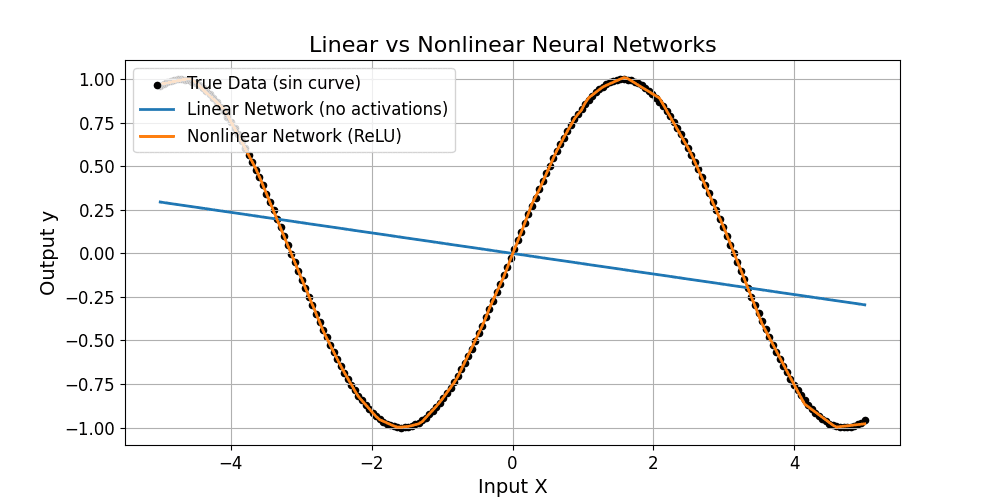
    Sine wave data with a deep linear network fitting only a straight line while a ReLU network tracks the curve

    Figure 1: The collapse in practice: on sine-wave data, a network without activations (blue) fits nothing but a straight line regardless of depth, while the same architecture with ReLU activations (orange) tracks the true curve (black dots) almost perfectly.


    Login to view more content