Tag: Kmeans

ML0094 GMM vs K-Means

How does Gaussian Mixture Model clustering differ from k-means, and why do production systems like speaker diarization prefer soft assignments?

Answer

A Gaussian Mixture Model is a probabilistic clustering model that represents the data as a weighted sum of K Gaussian distributions, each with its own mean, covariance, and mixing weight. Where k-means assigns each point to exactly one cluster (hard assignment) by nearest centroid, a GMM assigns each point a responsibility (posterior probability) for each cluster (soft assignment), so a point on the boundary between two clusters can be 60% in one and 40% in another. K-means is the limiting case of a GMM with shared spherical covariances as that shared variance goes to zero, which collapses the E-step posterior to an argmax. The GMM is fit by Expectation-Maximization: the E-step computes responsibilities, the M-step updates means, covariances, and mixing weights, iterating until convergence. Production systems use GMMs where uncertainty matters: joint diarization and separation systems pair a complex Angular Central Gaussian Mixture Model for source separation with a von Mises-Fisher mixture for diarization, so overlapping speech can be attributed to multiple speakers at once, and Flash-GMM (2026) made GMM training viable at 100x larger scale via fused Triton kernels.

(1) Hard vs Soft Assignment: k-means assigns each point to one centroid (argmin distance); GMM assigns a probability vector (responsibilities) across all clusters, so border points express uncertainty instead of being forced into one group.
(2) Spherical vs Elliptical Clusters: k-means assumes spherical, equally sized clusters (isotropic variance); GMM allows each cluster to have its own full covariance matrix, capturing elliptical and differently sized clusters.
(3) Production Soft Clustering: speaker diarization uses cACGMM and vMFMM mixture models so frame-level embeddings can belong to multiple speakers during overlap, and Flash-GMM’s fused Triton kernel achieved 20x speedup and 100x larger dataset scale, making soft GMM clustering a viable drop-in for k-means in approximate nearest-neighbor search with 2-12 point recall@10 gains.

Two panels: left shows k-means hard assignment with Voronoi boundaries and each point colored as one cluster; right shows GMM soft assignment with elliptical cluster contours and a border point labeled with 60/40 responsibility split

Figure 1: k-means forces each point into one cluster via nearest-centroid (hard assignment with spherical Voronoi cells), while a GMM assigns posterior probabilities (soft assignment) and can model elliptical clusters with per-component covariance matrices.

The EM algorithm for GMMs iterates two steps. In the E-step, each point’s responsibility for cluster k is computed as the posterior $\gamma_{ik} = \pi_k \mathcal{N}(x_i \mid \mu_k, \Sigma_k) / \sum_j \pi_j \mathcal{N}(x_i \mid \mu_j, \Sigma_j)$ . In the M-step, the parameters are updated: the mean is the responsibility-weighted average, the covariance is the responsibility-weighted scatter, and the mixing weight is the average responsibility. Each iteration is guaranteed never to decrease the log-likelihood, but it converges only to a local optimum, so multiple random restarts are standard. The key trade-off versus k-means is cost: k-means is O(nKd) per iteration with a simple distance computation, while GMM is O(nKd^2) per iteration because of the multivariate Gaussian PDF with full covariance, plus the matrix inversion in the PDF. Flash-GMM (2026) addressed this by eliminating the full responsibility matrix from GPU memory, reducing memory from O(nK) to O(KD) and enabling 100x larger datasets on a single GPU.

EM iteration flow: E-step computes responsibilities as posterior probabilities from current parameters, M-step updates means, covariances, and mixing weights from weighted statistics, with an arrow looping back to E-step until convergence

Figure 2: The EM loop for GMMs: the E-step computes soft responsibilities from current parameters, the M-step updates means, covariances, and mixing weights from responsibility-weighted statistics, and the cycle repeats until log-likelihood converges.

Mathematical Formulation:
$p(x) = \sum_{k=1}^{K} \pi_k\, \mathcal{N}(x \mid \mu_k, \Sigma_k)$
$\gamma_{ik} = \frac{\pi_k\, \mathcal{N}(x_i \mid \mu_k, \Sigma_k)}{\sum_{j=1}^{K} \pi_j\, \mathcal{N}(x_i \mid \mu_j, \Sigma_j)}$
$\mu_k = \frac{\sum_i \gamma_{ik}\, x_i}{\sum_i \gamma_{ik}},\quad \Sigma_k = \frac{\sum_i \gamma_{ik}\,(x_i - \mu_k)(x_i - \mu_k)^\top}{\sum_i \gamma_{ik}}$

Where:

$\pi_k$ is the mixing weight of cluster $k$ (prior probability, sums to 1), $\mu_k$ is its mean, and $\Sigma_k$ is its covariance matrix.
$\gamma_{ik}$ is the responsibility of cluster $k$ for point $i$ : the posterior probability that point $i$ was generated by component $k$ . This is the soft assignment that k-means replaces with a hard argmax.
The M-step updates are weighted by responsibilities: $\mu_k$ is the responsibility-weighted mean, $\Sigma_k$ is the responsibility-weighted covariance, and $\pi_k = \frac{1}{n}\sum_i \gamma_{ik}$ is the average responsibility. k-means is the limit when all $\Sigma_k = \sigma^2 I$ and $\sigma \to 0$ , collapsing responsibilities to 0 or 1.

Property	k-means	GMM
Assignment	Hard (argmin distance)	Soft (posterior responsibilities)
Cluster Shape	Spherical, equal variance	Elliptical, per-component covariance
Objective	Minimize within-cluster SSE	Maximize log-likelihood
Cost per Iteration	O(nKd)	O(nKd^2) with full covariance
Production Use	Vector quantization, image compression	Speaker diarization (cACGMM), ANN search (Flash-GMM)

August 12, 2026

ML0093 DBSCAN Clustering

How does DBSCAN work, and what advantages does it have over k-means for clustering tasks like geospatial stop detection?

Answer

DBSCAN is a density-based clustering algorithm: it groups points that are packed closely together and labels isolated points as noise, all without being told how many clusters to find. For each point it counts how many points fall within a radius eps; any point whose eps-neighborhood holds at least min_samples points (counting itself) is a core point, and clusters grow by linking core points whose neighborhoods overlap, then attaching their non-core neighbors. K-means, by contrast, requires you to specify K upfront and partitions data into Voronoi cells around centroids, which forces spherical clusters and assigns every point somewhere even if it is an outlier. In geospatial applications, DBSCAN is used to cluster raw GPS pings into “stops” because the density-based approach naturally absorbs GPS jitter and ignores transient traffic halts without needing a predefined polygon count.

(1) Density-Connected Expansion: a cluster is the maximal set of density-reachable points from a core point; points with fewer than min_samples neighbors but inside a core’s eps-radius become border points, and points reachable from no core become noise.
(2) No K and Arbitrary Shapes: DBSCAN discovers the cluster count from the data and follows winding, non-convex boundaries, which k-means cannot do because its Voronoi partition assumes spherical, similarly sized groups.
(3) Production Pattern: geospatial pipelines chain DBSCAN then SVM on GPS streams for foot-traffic analysis, and embedding-based clustering pairs UMAP with HDBSCAN (hierarchical DBSCAN) for recursive clustering because it handles varying densities and auto-selects stable clusters without an eps parameter.

Left panel: DBSCAN core point with eps-radius circle and min_samples neighbors, a border point on the circle edge, and a noise point outside; right panel: density-reachable expansion linking core points into an arbitrary-shaped cluster

Figure 1: DBSCAN mechanics: a core point has at least min_samples neighbors inside the eps-radius circle; clusters expand by chaining overlapping core neighborhoods, border points attach to one cluster, and isolated points become noise.

The practical trade-off is parameter sensitivity and density variation. DBSCAN’s eps must be tuned to the data’s scale, and a single global eps struggles when clusters have different densities, which is why HDBSCAN extends DBSCAN into a hierarchy and extracts stable clusters at varying density levels. K-means is cheaper at scale (each iteration is O(nKd) and embarrassingly parallel) and wins when clusters are genuinely spherical and K is known, as in vector quantization for image compression. DBSCAN’s neighborhood queries cost O(n log n) with a spatial index but degrade to O(n^2) in high dimensions where indexing breaks down, so production pipelines reduce dimensionality with UMAP first.

Two side-by-side panels on the same two-moon dataset: the left panel shows k-means cutting both moons with a straight dashed Voronoi boundary, the right panel shows DBSCAN recovering the two curved moons and marking sparse points as noise with gray crosses

Figure 2: On a non-convex two-moon dataset, k-means imposes a linear Voronoi cut that slices through both moons, while DBSCAN follows the curved density ridges and marks sparse-gap points as noise.

Mathematical Formulation:
$N_{\mathrm{eps}}(p) = \{q \in D \mid \mathrm{dist}(p, q) \leq \mathrm{eps}\}$
$\text{core}(p) \iff |N_{\mathrm{eps}}(p)| \geq \mathrm{min\_samples}$
$q \in C \iff \exists\, p_1, \ldots, p_t \in D:\ p_i \text{ core},\ p_{i+1} \in N_{\mathrm{eps}}(p_i),\ q \in N_{\mathrm{eps}}(p_t)$

Where:

$N_{\mathrm{eps}}(p)$ is the eps-neighborhood of point $p$ in dataset $D$ , and $\mathrm{dist}$ is typically Euclidean distance.
A point is core when its neighborhood contains at least min_samples points; border points are in a core’s neighborhood but are not core themselves; noise points are in no core’s neighborhood.
A cluster $C$ is the maximal set of points density-reachable from a core point via a chain of overlapping core neighborhoods; this transitive closure is what lets DBSCAN trace arbitrary shapes.

Property	DBSCAN	k-means
Cluster Count	Discovered from density; no K needed	Must specify K upfront
Cluster Shape	Arbitrary, density-connected	Spherical Voronoi cells
Outliers	Labeled as noise explicitly	Force-assigned to nearest centroid
Parameters	eps, min_samples	K, initialization
Scalability	O(n log n) with spatial index; O(n^2) worst case	O(nK) per iteration, parallelizable
Weakness	Single eps fails on varying densities (HDBSCAN fixes this)	Breaks on non-spherical or unequal-size clusters

August 12, 2026

ML0061 KNN and K-means

What are the key differences between KNN and K-means?

Answer

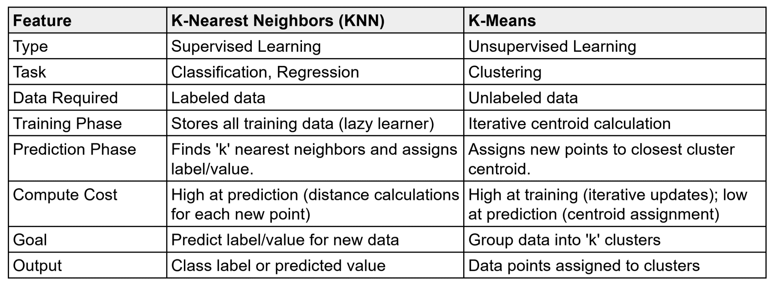
KNN (K-Nearest Neighbors) is a supervised algorithm that classifies data using the labels of its nearest neighbors: prediction from historical labeled data. K-means is an unsupervised clustering technique that groups data purely by similarity, using no labels at all. Despite the shared “K”, they solve different problems.

(1) Learning Type: KNN is supervised (classification/regression); K-means is unsupervised (clustering).
(2) Objective: KNN predicts a new sample’s label from the majority vote (or average) of its K nearest neighbors; K-means partitions the dataset into K clusters by minimizing intra-cluster distance.
(3) Training: KNN has no explicit training: it stores the entire dataset; K-means iteratively learns cluster centroids.
(4) Prediction Cost: KNN is expensive at prediction (distance to every training point, sort, take the top K, then vote/average); K-means is cheap: distances to K centroids, assign the nearest.
(5) Distance Use And Output: KNN uses distance to find neighbors and outputs a label or value; K-means uses distance to assign points to centroids and outputs cluster assignments plus centroids.

Feature	K-Nearest Neighbors (KNN)	K-Means
Type	Supervised Learning	Unsupervised Learning
Task	Classification, Regression	Clustering
Data Required	Labeled data	Unlabeled data
Training Phase	Stores all training data (lazy learner)	Iterative centroid calculation
Prediction Phase	Finds K nearest neighbors and assigns label/value	Assigns new points to closest cluster centroid
Compute Cost	High at prediction (distance calculations for each new point)	High at training (iterative updates); low at prediction (centroid assignment)
Goal	Predict label/value for new data	Group data into K clusters
Output	Class label or predicted value	Data points assigned to clusters

Mathematical Formulation:
$\hat{y} = \arg\max_{c \in \mathcal{C}} \; \sum_{i=1}^{K} \mathbb{1}(y_i = c)$
$\min_{C_1, \ldots, C_K} \; \sum_{k=1}^{K} \sum_{x \in C_k} \|x - \mu_k\|^2$

Where:

KNN (first line): $\hat{y}$ is the predicted class, $\mathcal{C}$ the class set, $y_i$ the label of the $i$ -th nearest neighbor, and $\mathbb{1}(\cdot)$ the vote-counting indicator.
K-means (second line): $C_k$ is cluster $k$ and $\mu_k$ its centroid; the algorithm minimizes total within-cluster squared distance: no labels appear anywhere.

Two panels on crescent moon data showing KNN separating the moons correctly while K-means cuts through them

Figure 1: Same data, different goals: with labels, KNN’s local votes trace the two crescents perfectly (left); without labels, K-means can only split by nearest-centroid geometry and slices through both moons (right). KNN performs well here thanks to local decision-making; K-means fails because it assumes spherical clusters with linear boundaries.

June 18, 2025

ML0060 K Selection in K-Means
How to select K in K-Means?
Answer
To select the optimal number of clusters $K$ in K-means, combine visual tools (the elbow method), quantitative metrics (the silhouette score), and statistical methods (the gap statistic), balancing model fit against generalization without overfitting. Domain knowledge and interpretability should have the final word.
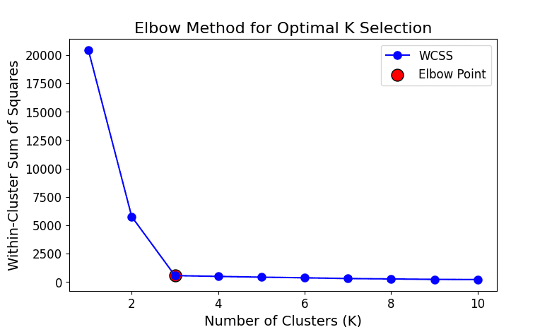
(1) Elbow Method: Plot within-cluster sum of squares (WCSS) against $K$ and pick the “elbow” where the rate of improvement sharply slows.
(2) Silhouette Score: Compute the average silhouette coefficient for each candidate $K$ and pick the highest: it rewards tight, well-separated clusters.
(3) Gap Statistic: Compare the observed WCSS against that of a random reference distribution; pick the $K$ maximizing the gap.

Figure 1: The elbow method: WCSS always decreases as K grows, but the marginal gain collapses after the true cluster count (the marked elbow at K = 3). Beyond the elbow you pay model complexity for noise.
Mathematical Formulation:
$\text{WCSS}(K) = \sum_{k=1}^{K} \sum_{x_i \in C_k} \|x_i - \mu_k\|^2$
$s(i) = \frac{b(i) - a(i)}{\max\big(a(i),\, b(i)\big)}$
Where:
$C_k$ is cluster $k$ and $\mu_k$ its centroid; WCSS is the total within-cluster squared distance that the elbow method plots against $K$ .
$a(i)$ is point $i$ ‘s mean distance to its own cluster (intra-cluster); $b(i)$ its mean distance to the nearest other cluster.
$s(i) \in [-1, 1]$ : near 1 means well clustered, near 0 means on a boundary, negative means likely misassigned; average it over all points for each $K$ .
Login to view more content
June 14, 2025
ML0059 K-means II
K-Means is widely used for clustering. Can you discuss its main benefits as well as its disadvantages?
Answer
K-means partitions data into $K$ clusters where each point belongs to the cluster with the nearest mean. It is computationally efficient and easy to implement, but it requires specifying the number of clusters in advance, assumes spherical clusters, and is sensitive to initialization and outliers.
(1) Simple And Efficient: Fast to compute, easy to implement, and scalable to large datasets.
(2) Unsupervised And Interpretable: Needs no labels, and the centroids are intuitive summaries of each cluster.
(3) Strong Assumptions: Works best on compact, well-separated spherical clusters; the user must fix $K$ beforehand.
(4) Fragility: Poor initial centroids can lock in suboptimal results, outliers drag centroids, and plain Euclidean distance excludes non-numeric features.
Mathematical Formulation:
$J = \sum_{i=1}^{K} \sum_{x_j \in C_i} \|x_j - \mu_i\|^2$
Where:
$K$ is the number of clusters; $C_i$ the set of points in cluster $i$ .
$\mu_i$ is the centroid of cluster $i$ ; $x_j$ a data point assigned to it.
$J$ is the within-cluster sum of squared distances: the objective both steps of the algorithm drive down monotonically.

Figure 1: The assumption made visible: on spherical, well-separated blobs (left) K-means nails the structure; on two crescents (right) its linear, centroid-based split slices through both moons: the spherical-cluster assumption failing in action.
Login to view more content
June 12, 2025
ML0058 K-means++
Please explain how K-means++ works.
Answer
K-means++ is an improved way to initialize the centroids of K-means. Instead of picking all centroids uniformly at random, it selects them one by one with probability proportional to the squared distance from the already chosen centroids. This spreads the initial centroids out, sharply reducing the chance of poor clustering and helping the algorithm converge faster and more reliably. After initialization, standard K-means proceeds unchanged.
(1) First Centroid: Choose $\mu_1$ uniformly at random from the dataset.
(2) Distance Computation: For each point, compute its squared distance to the nearest already-chosen centroid.
(3) Weighted Selection: Pick the next centroid with probability proportional to that squared distance: far points are favored.
(4) Repeat Until K: Continue until all $K$ centroids are chosen, then run standard K-means.

Figure 1: K-means++ initialization (K=5): the distance-squared weighting spreads the starting centroids across all five natural groups, so the algorithm starts close to a good solution instead of gambling on random seeds.
Mathematical Formulation:
$D(x_i)^2 = \min_{1 \le j \le m} \|x_i - \mu_j\|^2$
$P(x_i) = \frac{D(x_i)^2}{\sum_j D(x_j)^2}$
Where:
$\mu_j$ is one of the $m$ already chosen centroids; $D(x_i)^2$ is point $x_i$ ‘s squared distance to its nearest chosen centroid.
$P(x_i)$ is the probability of $x_i$ becoming the next centroid, proportional to $D(x_i)^2$ , so points far from every chosen centroid are exponentially favored over nearby ones.
The denominator normalizes over all data points; selection repeats until $K$ centroids exist.

Figure 2: Why initialization matters: with an unlucky random init (left), two centroids land in one group and the small top cluster is merged away; K-means++ (right) seeds one centroid per group and recovers all three clusters cleanly.
Login to view more content
June 12, 2025
ML0057 K-means
Please explain how K-means works.
Answer
K-means is an iterative unsupervised algorithm that partitions data into $K$ clusters by minimizing intra-cluster distances (within-cluster variance). It alternates between assigning points to the nearest centroid and recomputing centroids until convergence. It is fast and easy to implement, but sensitive to initialization and to non-convex cluster shapes.
(1) Initialization: Choose $K$ initial centroids (randomly, or with K-means++).
(2) Assignment Step: Assign every point to its closest centroid by Euclidean distance.
(3) Update Step: Recompute each centroid as the mean of the points assigned to it.
(4) Convergence: Repeat assignment and update until the centroids stabilize or a stopping criterion is met.

Figure 1: K-means (K=3) converged on blob data: colors mark the final assignments and the red X’s are the centroids: each is the mean of its cluster, and every point belongs to its nearest centroid’s cluster.
Mathematical Formulation:
$d(x, c_k) = \sqrt{\sum_{i=1}^{n} (x_i - c_{k,i})^2}$
$c_k = \frac{1}{|C_k|} \sum_{x \in C_k} x$
Where:
$x$ is a data point and $c_k$ the centroid of cluster $k$ (first formula: Euclidean assignment distance, $n$ = number of features).
$C_k$ is the set of points currently assigned to cluster $k$ ; the update sets the centroid to their component-wise mean, the minimizer of squared distances for a fixed assignment.
Login to view more content
June 12, 2025