Tag: Norm

DL0065 Group Normalization
What is Group Normalization?
Answer
Group Normalization normalizes each sample independently by dividing its channels into groups and computing a mean and variance over the channels and spatial positions within each group. The normalized activations then receive learned per-channel scale and shift parameters. Because its statistics do not depend on other examples, GroupNorm behaves consistently with very small or variable batch sizes and uses the same computation during training and inference. The group count must be compatible with the channel count, and its inductive bias can be less suitable than BatchNorm when large, stable batches provide useful batch statistics.
(1) Per-Sample Statistics: Each example has its own group means and variances, so no running batch averages are required.
(2) Channel Grouping: For $C$ channels and $G$ groups, each group normalizes $(C/G)\times H\times W$ values; channels within a group share statistics.
(3) Boundary Cases: $G=1$ normalizes all channels and spatial positions together, while $G=C$ gives one channel per group and resembles InstanceNorm.

Figure 1: A convolutional tensor is split into channel groups; each sample-group gets independent statistics before per-channel affine scaling.
Mathematical Formulation:
$\mu_{n,g}=\frac{1}{m}\sum_{i\in S_{n,g}}x_i$
$\sigma^2_{n,g}=\frac{1}{m}\sum_{i\in S_{n,g}}(x_i-\mu_{n,g})^2$
$y_{n,c,h,w}=\gamma_c\frac{x_{n,c,h,w}-\mu_{n,g(c)}}{\sqrt{\sigma^2_{n,g(c)}+\epsilon}}+\beta_c$
Where:
$n$ indexes samples, $g$ indexes channel groups, and $c,h,w$ index channel and spatial position.
$S_{n,g}$ is the set of activations in group $g$ of sample $n$ ; $i$ indexes elements in that set.
$m=(C/G)HW$ is the number of normalized values when $C$ channels are divided into $G$ groups over height $H$ and width $W$ .
$\mu_{n,g}$ and $\sigma^2_{n,g}$ are the group mean and variance; $x$ and $y$ are input and normalized output activations.
$g(c)$ maps channel $c$ to its group, $\gamma_c,\beta_c$ are learned per-channel scale and shift, and $\epsilon$ stabilizes division.

Figure 2: Normalization families differ mainly in which batch, channel, and spatial axes share statistics and whether inference needs running estimates.
Login to view more content
July 20, 2026
DL0034 Layer Norm
What is layer normalization, and why is it used in Transformers?
Answer
Layer Normalization (LN) standardizes the features of each individual sample: for one token’s embedding vector, it computes the mean and variance across the feature dimension only, rescales to zero mean and unit variance, then applies a learnable scale and shift. Unlike BatchNorm, it never looks across the batch, which is exactly why Transformers, with variable-length sequences and small or on-the-fly batches, rely on it in every block.
(1) Normalization Within a Sample: Mean and variance come from the $d_{model}$ features of a single token: one set of statistics per token, not per batch.
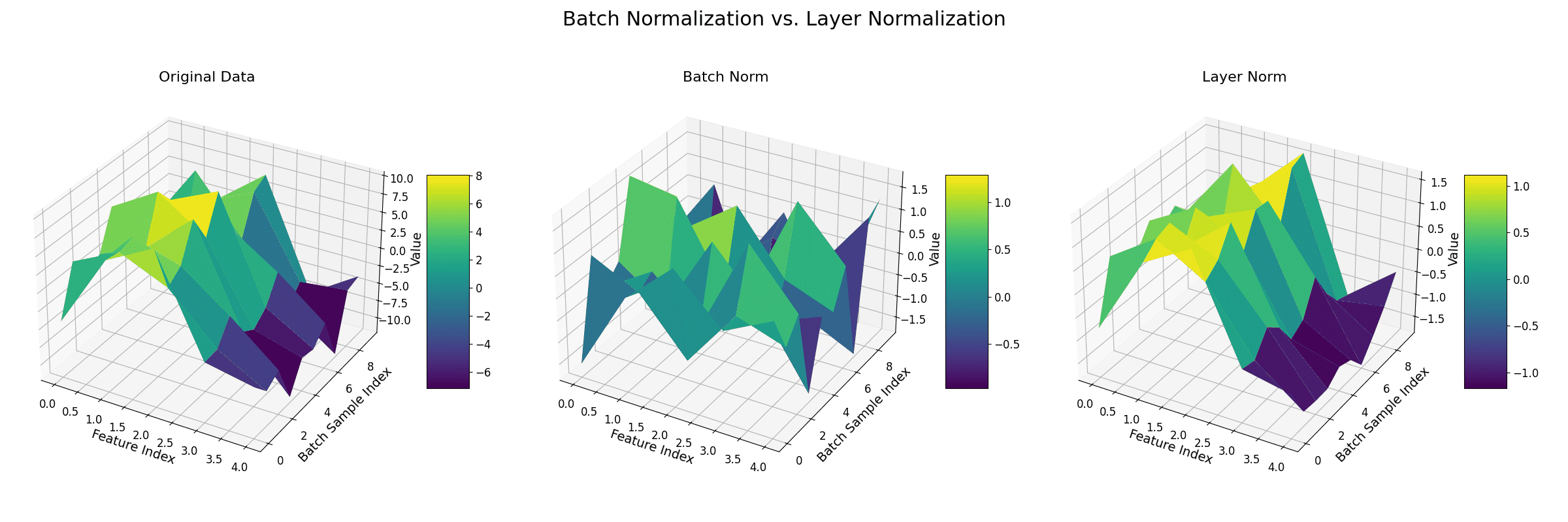
(2) Batch-Size Independence: Behavior is identical at train and test time and for any batch size: no running statistics, no mismatch.
(3) Stabilizes Training: Keeps activations in a consistent range, preventing exploding/vanishing gradients and enabling deep stacks to converge faster.

Figure 1: Layer Normalization standardizes each sample (row) across its own feature dimensions; statistics never cross sample boundaries, so batch size is irrelevant.
Mathematical Formulation:
$\hat{x}_i = \frac{x_i - \mu}{\sqrt{\sigma^2 + \epsilon}} \cdot \gamma + \beta$
$\mu = \frac{1}{d}\sum_{i=1}^{d} x_i$
$\sigma^2 = \frac{1}{d}\sum_{i=1}^{d}(x_i - \mu)^2$
Where:
$x_i$ is one feature of a single token’s $d$ -dimensional vector; statistics are computed over $i = 1..d$ for that token alone.
$\epsilon$ is a small constant for numerical stability; $\gamma, \beta$ are learnable per-feature scale and shift that restore representational freedom.
Why Not BatchNorm: BatchNorm’s statistics mix information across samples, degrade with small or variable-size batches, behave differently at train vs inference, and pad tokens corrupt the per-feature means of variable-length sequences: all fatal for typical Transformer workloads.

Figure 2: Placement variants: original Post-LN (after the residual add) vs modern Pre-LN (inside the residual branch), which keeps a clean gradient highway.
Where It Sits: Every attention and FFN sub-layer is wrapped as $\mathrm{LN}(x + \mathrm{Sublayer}(x))$ (Post-LN) in the original paper; most modern LLMs use Pre-LN, normalizing the sub-layer input instead, which trains stably even without learning-rate warmup.
Login to view more content
August 14, 2025

DL0013 Instance Normalization

Can you explain what Instance Normalization is in the context of deep learning?

Answer

Instance Normalization (IN) normalizes each individual sample and each channel independently: for every (instance, channel) pair it subtracts the mean and divides by the standard deviation computed over that feature map’s spatial dimensions only. Because statistics never cross instance boundaries, IN is unaffected by mini-batch composition and works with batch size 1. This per-instance normalization removes sample-specific contrast and style, which is why IN became the standard in style transfer and image-generation models.

(1) Per-Instance, Per-Channel Statistics: Mean and variance are computed over the $H \times W$ spatial positions of each channel of each sample separately, so no information leaks across the batch.
(2) Batch-Size Independent: Statistics do not depend on other samples, so IN behaves identically at training and test time and remains stable with small batches.
(3) Removes Instance-Specific Style: Normalizing each map’s contrast discards style-like appearance information while preserving content structure, which suits style transfer, GANs, and domain adaptation.

Side-by-side diagram of batch normalization sharing per-channel statistics across all instances versus instance normalization computing statistics within each instance-channel feature map.

Figure 1: BN pools statistics per channel across the whole batch (red dashed groups), while IN normalizes each (instance, channel) map alone (orange dashed boxes): the source of IN’s batch independence.

Mathematical Formulation:
$\mu_{nc} = \frac{1}{HW} \sum_{h=1}^{H} \sum_{w=1}^{W} x_{nchw}$
$\sigma_{nc}^2 = \frac{1}{HW} \sum_{h=1}^{H} \sum_{w=1}^{W} (x_{nchw} - \mu_{nc})^2$
$\hat{x}_{nchw} = \frac{x_{nchw} - \mu_{nc}}{\sqrt{\sigma_{nc}^2 + \epsilon}}$
$y_{nchw} = \gamma_c\,\hat{x}_{nchw} + \beta_c$

Where:

$x_{nchw}$ is the input activation at batch index $n$ , channel $c$ , spatial position $(h, w)$ .
$\mu_{nc}$ and $\sigma_{nc}^2$ are the mean and variance over the $H \times W$ spatial extent of instance $n$ , channel $c$ .
$\hat{x}_{nchw}$ is the normalized activation; $\epsilon$ is a small constant for numerical stability.
$\gamma_c$ and $\beta_c$ are learnable per-channel scale and shift parameters; $y_{nchw}$ is the output.

Contrast with Batch Normalization: BN computes per-channel statistics over the entire mini-batch ( $N \times H \times W$ ), which couples a sample’s output to its batchmates and forces a switch to running averages at inference. IN’s per-sample statistics are identical in both phases, and discarding per-instance contrast is precisely what removes style from content images.

Feature	Instance Normalization (IN)	Batch Normalization (BN)
Scope of stats	Per instance, per channel (over $H \times W$ )	Per channel (over $N \times H \times W$ )
Batch size	Independent; works with batch = 1	Dependent; needs stable batch stats
Primary use	Style transfer, GANs, domain adaptation	Image classification, general CNNs
Effect	Removes instance-specific style/contrast	Stabilizes training, speeds convergence
Inference	Same per-sample stats at test time	Uses running stats from training

Bottom line: IN removes per-instance contrast (style); BN aligns feature scales across the batch. IN trades BN’s cross-sample regularization for batch independence and style removal.

May 22, 2025

DL0007 Batch Norm
Why use batch normalization in deep learning training?
Answer
Batch normalization stabilizes and accelerates training by normalizing each layer’s inputs across the mini-batch: subtract the batch mean and divide by the batch standard deviation. After normalization, a learnable scale $\gamma$ and shift $\beta$ let the network recover the identity transformation if needed. BN is applied after the linear transform (e.g., the convolution) and before the activation (e.g., ReLU).
(1) Stabilizes Learning: Reduces internal covariate shift, making training less sensitive to initialization and hyperparameter choices.
(2) Enables Higher Learning Rates: Larger learning rates can be used without instability, leading to faster convergence.
(3) Improves Generalization: Normalizing per mini-batch introduces noise into activations, preventing over-reliance on specific batches and acting as a mild regularizer.

Figure 1: Each feature channel is normalized using its mini-batch statistics, then rescaled by learnable $\gamma$ and $\beta$ .
Mathematical Formulation:
$BN(x_i) = \gamma \left( \frac{x_i - \mu_B}{\sqrt{\sigma_B^2 + \epsilon}} \right) + \beta$
Where:
$x_i$ is an individual feature value in the batch.
$\mu_B$ and $\sigma_B^2$ are the mean and variance of that feature across the current mini-batch.
$\epsilon$ is a small constant (e.g., $10^{-5}$ ) added for numerical stability.
$\gamma$ and $\beta$ are learnable scaling and shifting parameters.

Figure 2: Training computes per-batch statistics and updates running averages; inference uses the frozen running averages, producing deterministic outputs.
Placement in a CNN Block: BN sits between the linear transform and the non-linearity: Conv2D → BatchNorm → ReLU.

Figure 3: In a standard CNN block, BatchNorm normalizes the convolution output before the activation function.
Login to view more content
April 30, 2025
ML0018 Data Normalization
Why is data normalization used in Machine Learning?
Answer
Data normalization scales features into a specific range or distribution: typically [0, 1] with min-max scaling, or mean 0 and standard deviation 1 with standardization, so that every feature contributes comparably to learning. It is used for three reasons. First, better model performance: algorithms built on distance metrics, such as k-nearest neighbors and SVMs, are skewed when one feature spans thousands and another spans decimals, normalization puts them on the same scale. Second, training stability and speed: normalized inputs keep neural network gradients well-conditioned, so training converges faster and more smoothly. Third, fair feature contribution: without scaling, large-magnitude features dominate the objective while small-magnitude ones are ignored, regardless of how informative they actually are.
(1) What It Does: Rescales each feature to a common range (min-max) or distribution (z-score standardization).
(2) Who Needs It: Distance-based models (kNN, SVM), gradient-based learners (neural networks, linear/logistic regression); tree ensembles largely do not.
(3) The Payoff: Faster convergence, stabler training, and features competing on information rather than magnitude.

Figure 1: Before: one axis spans hundreds while the other spans decimals, so distance is decided by the big axis alone. After standardization, both features contribute equally.
Mathematical Formulation:
$x' = \frac{x - x_{\min}}{x_{\max} - x_{\min}}$
$z = \frac{x - \mu}{\sigma}$
Where:
$x'$ is the min-max normalized value of feature value $x$ , squashed into [0, 1].
$x_{\min}$ and $x_{\max}$ are the feature’s minimum and maximum computed on the training set only.
$z$ is the standardized (z-score) value with mean 0 and standard deviation 1.
$\mu$ and $\sigma$ are the feature’s training-set mean and standard deviation; fitting them on all data would leak test information.
Login to view more content
March 28, 2025

Tag: Norm

DL0065 Group Normalization

DL0034 Layer Norm

DL0013 Instance Normalization

DL0007 Batch Norm

ML0018 Data Normalization