Tag: VLM

Vision-Language Models (multimodal understanding)

DL0179 Grounding DINO vs Faster R-CNN

How does Grounding DINO’s open-vocabulary object detection, which conditions on free-form text, differ from classic Faster R-CNN’s closed-category detection in architecture, training data, and deployment flexibility?

Answer

Faster R-CNN is a closed-set detector: the label space is baked into a final linear layer of shape $(K+1) \times d$ , so the model can only ever emit one of the $K$ categories it was trained on plus background. Grounding DINO keeps the same output contract (boxes with scores) but deletes that fixed head and replaces it with a region-text similarity. A prompt such as “dog . traffic cone .” is encoded by BERT, its token features are fused with image features in three places (the neck feature enhancer, the language-guided query selection stage, and the cross-modality decoder), and each of the 900 decoder queries is scored by a dot product against every text token instead of by a softmax over classes. Because the class list moved out of the weight matrix and into the input, adding a category becomes a string edit rather than an annotation, retraining, and redeployment cycle. The bill arrives in training data (detection plus grounding plus caption-derived boxes instead of one boxed dataset) and in inference cost (a transformer detector with a text encoder instead of a ResNet with a two-layer head).

(1) Fixed Head vs Contrastive Alignment: Faster R-CNN classifies with $\mathrm{softmax}(W f_i + b)$ over $K+1$ rows; Grounding DINO scores each query against each text token and applies a sigmoid per pair, so categories do not compete for a shared probability mass.
(2) Text Is An Input, Not A Label Set: the prompt is runtime configuration, which means the same weights detect “forklift” today and “spilled pallet” tomorrow with no gradient step.
(3) Fusion Happens Early And Often: a late-fusion design that only compares final features would leave the proposal stage text-blind, so Grounding DINO injects language into the encoder, into query selection, and into the decoder.
(4) Detector Family Differs Too: anchors, RoIAlign, and NMS are replaced by DETR-style one-to-one Hungarian matching with learned queries, which removes the anchor and NMS hyperparameters but slows convergence.
(5) Training Data Is The Real Difference: COCO’s 80 categories over ~118k images versus a mixture of Objects365, GoldG, and caption-mined pseudo boxes covering tens of thousands of phrase types.
(6) Flexibility Costs Latency And Calibration: open-vocabulary scores are per-phrase and poorly comparable across phrases, so thresholds must be tuned per prompt rather than set once.

Side-by-side vertical pipelines: left panel shows Faster R-CNN with image only, ResNet-50 plus FPN, Region Proposal Network producing about a thousand proposals, RoIAlign with a two-FC box head, and a softmax over K plus one fixed classes followed by NMS; right panel shows Grounding DINO with two input lanes for image and text prompt, a Swin backbone and a BERT text encoder, a feature enhancer combining deformable self-attention with bi-directional image-text cross-attention, language-guided query selection producing 900 cross-modality queries, and a cross-modality decoder emitting region-text contrastive logits whose label space is the prompt

Figure 1: The vocabulary lives in a different place. On the left it is a row of $W$ ; on the right it is a string that enters the network beside the pixels, so language influences which regions are proposed at all, not only how a finished proposal is labeled.

The training recipe follows from that architecture. Faster R-CNN needs one homogeneous boxed dataset, and every category must appear with exhaustive box annotation, which is why closed-set benchmarks stall around a few hundred classes. Grounding DINO is trained on a mixture of supervision grades: fully annotated detection data (COCO, Objects365 with 365 categories), human phrase grounding data (GoldG, built from Flickr30k Entities and Visual Genome), and caption data whose boxes are pseudo-labeled by a teacher in the GLIP lineage. The reformulation that makes this legal is treating detection as grounding: a detection dataset is just a caption of concatenated category names, so a single per-token alignment loss (focal loss on region-token logits) consumes all three grades plus the usual $L_1$ and GIoU box terms. The payoff is that a Swin-T model reaches about 48.4 AP zero-shot on COCO without seeing a single COCO image, and roughly 27 AP on LVIS minival where the long tail is exactly what a fixed 80-way head cannot express.

Mathematical Formulation:
$p_i = \mathrm{softmax}(W f_i + b)$
$W \in \mathbb{R}^{(K+1) \times d}$
$s_{ij} = q_i^{\top} t_j$
$\hat{p}_{ij} = \sigma(s_{ij})$
$s_i(P) = \max_{j \in P} s_{ij}$

Where:

$p_i$ is the closed-set posterior for RoI $i$ over $K+1$ outcomes, and $f_i \in \mathbb{R}^{d}$ is its pooled RoIAlign feature; the row count of $W$ is the vocabulary, which is why the label space is a weight-shape decision.
$q_i \in \mathbb{R}^{d}$ is the $i$ -th decoder query (Grounding DINO uses $N_q = 900$ ) and $t_j \in \mathbb{R}^{d}$ is the $j$ -th projected text token feature; both are projected into one shared embedding space, so the dot product is directly the logit.
$\sigma$ is the sigmoid, so every region-token pair is an independent binary decision; nothing forces the scores of a query to sum to one across the prompt.
$P$ is the set of sub-word indices belonging to one phrase, and $s_i(P)$ is the phrase-level score obtained by taking the maximum over that phrase’s tokens.
Index ranges are $i \in \{1,\ldots,N_q\}$ and $j \in \{1,\ldots,L_t\}$ with $L_t \leq 256$ BERT sub-word tokens, which is the hard cap on how large a prompt vocabulary can be in one forward pass.

Two-panel figure: left panel is a grayscale bar chart of a Faster R-CNN softmax over person, car, dog, chair, tv, and background probabilities that sum to one, annotated that traffic cone has no column so mass is forced onto the nearest in-vocabulary class; right panel is a grayscale heatmap of sigmoid alignment scores between four decoder queries and the seven prompt sub-word tokens of dog . traffic cone . leash ., with high values where the cone query meets traffic and cone, the dog query meets dog, and the leash query meets leash, and near-zero values for the pavement query

Figure 2: Two different score semantics. The closed-set head must spend all probability mass inside its vocabulary, so an unseen object is mislabeled with confidence; the contrastive head gives each query an independent score per token, and a new phrase adds a column rather than a retrained row of $W$ .

Deployment flexibility is therefore real but not free. The prompt format matters: phrases are period-separated and Grounding DINO uses sub-sentence masking so unrelated category names do not attend to each other, yet cramming hundreds of categories into 256 tokens still degrades both accuracy and score calibration, and long or rare names fragment into sub-words whose max-pooled score behaves differently from a short common noun. Because $\hat{p}_{ij}$ is not normalized across phrases, a single global confidence threshold that is right for “person” is usually wrong for “loose cable”, so production systems keep a per-phrase threshold table. The common industrial pattern is not to serve the open-vocabulary model at all: use it plus a segmenter as an auto-labeler to bootstrap a dataset, then train or distill a fast closed-set detector for the frames-per-second and cost envelope the product actually needs.

Property	Faster R-CNN (closed set)	Grounding DINO (open vocabulary)
Label space	Rows of the classifier weight matrix, fixed at training time	Tokens of the prompt, chosen per request
Localization mechanism	Anchors, RPN proposals, RoIAlign, NMS at inference	900 learned queries, language-guided query selection, one-to-one Hungarian matching, no NMS
Classification	Softmax cross-entropy over $K+1$ classes	Focal loss on per-token region-text logits, sigmoid per pair
Training data	One exhaustively boxed dataset (COCO: 80 classes, ~118k images)	Detection (Objects365, 365 classes) plus grounding (GoldG) plus caption-mined pseudo boxes
Adding one category	Annotate, grow the head by about 5.1k parameters, retrain, revalidate, redeploy	Edit the prompt string, zero new parameters, no retraining
Reported accuracy	About 40 box AP on COCO with R50-FPN, undefined outside its 80 classes	48.4 AP zero-shot COCO and 57.2 AP fine-tuned with Swin-T; 52.5 AP zero-shot with Swin-L
Inference cost	Convolutional backbone plus a two-FC head, edge-deployable, easy to quantize	Transformer detector plus a text encoder; prompt features are cacheable when the vocabulary is fixed
Dominant failure mode	Confidently mislabels unseen objects as the nearest known class	Prompt-sensitive, per-phrase thresholds, degradation past the 256-token prompt budget

August 19, 2026

DL0177 Discrete vs Continuous Visual Tokens

What is the difference between discrete visual tokenization (e.g., VQ-VAE, VQ-GAN) and continuous vision embeddings (e.g., ViT patch outputs), and when is each preferred for generation versus understanding tasks?

Answer

Both paths begin identically, with a convolutional or ViT encoder turning the image into a grid of $d$ -dimensional vectors. The only structural difference is whether a quantizer follows. A discrete tokenizer (VQ-VAE, VQ-GAN) snaps each vector to its nearest entry in a learned codebook of $K$ vectors and keeps only the integer index, so an image becomes a string of ids over a finite vocabulary that a jointly trained decoder can invert back to pixels. A continuous representation (ViT patch outputs, CLIP or SigLIP features, KL-VAE latents) keeps the float vector, which preserves far more information but has no finite support, so no softmax and no cross-entropy can be defined over it. That single difference decides the downstream interface: discrete ids plug into next-token or masked-token prediction with exactly the machinery used for text, while continuous features must be projected into an LLM or denoised by a diffusion model. As a default, understanding prefers continuous features because quantization discards the high-frequency detail that OCR and fine-grained VQA depend on, while generation historically preferred discrete tokens because a categorical likelihood is easy to train and easy to sample.

(1) Only The Quantizer Differs: the encoder, the patch grid, and the spatial downsampling factor can be identical; adding a nearest-code lookup converts a float grid into an id grid.
(2) Information Budget: a discrete token carries $\log_2 K$ bits (10 to 18 in practice), while a continuous patch vector carries roughly $d \times 16$ bits of activation, three orders of magnitude more.
(3) Gradient Path: $\arg\min$ is non-differentiable, so VQ needs a straight-through estimator plus codebook and commitment losses, whereas continuous encoders train by plain backpropagation.
(4) Reconstruction Cost: heavy compression makes plain L2 reconstruction blurry, which is why VQ-GAN adds perceptual and patch-GAN losses to keep 16x-downsampled decodes sharp.
(5) Downstream Interface: discrete gives one softmax vocabulary shared with text; continuous gives features for a projector, cross-attention, or a latent diffusion denoiser.
(6) Task Split: continuous features dominate VLM understanding benchmarks; discrete tokens dominate when the goal is a single unified next-token model that also emits pixels.

Two horizontal pipelines: the upper understanding path runs input image to ViT patch encoder to 256 continuous vectors in R^1024 to a linear projector to an LLM emitting text, with no quantizer and no pixel decoder; the lower generation path runs input image to a CNN or ViT encoder to a quantizer that picks the nearest of K codes, to a 16 by 16 grid of integer ids, to a transformer with a softmax over K, to a decoder producing pixels

Figure 1: The same encoder, two endings. Deleting the quantizer leaves continuous features that a projector feeds to an LLM; inserting it buys a finite vocabulary and a pixel decoder at the price of $\log_2 K$ bits per token. Note that the understanding path has no decoder at all, which is why an understanding-only encoder is never required to be invertible.

The practical difficulty of discrete tokenization is that the codebook must be learned through a non-differentiable lookup. The straight-through estimator simply copies the decoder gradient past the quantizer, which is a biased estimate that works only if the encoder output stays close to its assigned code, hence the commitment loss. The characteristic failure is codebook collapse: a few entries win most assignments, the rest receive no gradient and die, and effective vocabulary size stops tracking nominal $K$ . Standard mitigations are EMA codebook updates, low-dimensional $\ell_2$ -normalized codes, dead-code re-initialization, and an entropy bonus on the assignment distribution. Continuous encoders have none of this machinery, but they also cannot be sampled from, since there is no distribution over $\mathbb{R}^{d}$ that a softmax can express, which is precisely why continuous-latent generation requires a diffusion or flow model rather than a token classifier.

Mathematical Formulation:
$z = E(x)$
$k = \arg\min_{j} \lVert z - e_j \rVert_2$
$z_q = e_k$
$\hat{x} = D(z_q)$
$\mathcal{L}_{\mathrm{com}} = \beta \lVert z - \mathrm{sg}(e_k) \rVert_2^2$

Where:

$x$ is the input image, $E$ the encoder, and $z \in \mathbb{R}^{d}$ one continuous patch vector from the encoder grid; keeping $z$ and stopping here is the continuous path.
$e_j$ for $j \in \{1,\ldots,K\}$ are the learned codebook vectors, $k$ is the selected index (the actual token), and $K$ is the vocabulary size.
$z_q$ is the quantized vector fed to the decoder $D$ , and the residual $z - z_q$ is information the model can never recover.
$\mathrm{sg}(\cdot)$ is the stop-gradient operator and $\beta$ (typically $0.25$ ) weights the commitment loss that pulls encoder outputs toward their assigned codes.
The full VQ-GAN objective adds a reconstruction term, an LPIPS perceptual term, and a patch-discriminator term to $\mathcal{L}_{\mathrm{com}}$ ; only the reconstruction term survives in a plain VQ-VAE.

Bit Budget For One 256×256 Image:
$B_{\mathrm{disc}} = 256 \times 14 = 3584$
$B_{\mathrm{cont}} = 256 \times 1024 \times 16$
$B_{\mathrm{cont}} = 4194304$
$B_{\mathrm{cont}} / B_{\mathrm{disc}} \approx 1170$

All four numbers are in bits. A 16x-downsampling tokenizer with $K = 16384$ compresses the image to 256 ids of 14 bits each, about 448 bytes, while a ViT-L/14 tower keeps 256 patch vectors of 1024 bf16 activations, about 512 KiB. That ratio is the whole argument: it is why a discrete sequence is short enough to model autoregressively alongside text, and equally why an OCR-heavy or chart-reading task should not be routed through it.

Left panel shows a two-dimensional scatter of continuous encoder outputs partitioned into nine square cells by dashed boundaries, with a black X codebook entry at each cell center and one highlighted red point joined by an arrow to its nearest code, labelled quantization error. Right panel plots reconstruction FID against bits per token from 10 to 18, with a plain VQ curve that stalls near 5 and rises after 14 bits, a lookup-free or FSQ curve that keeps falling toward 1.2, and a dashed horizontal line marking the continuous KL-VAE floor near 0.74

Figure 2: Left, quantization is a Voronoi partition of the latent space: the id names the cell, and the offset inside the cell is thrown away. Right, approximate published reconstruction results show that a plain VQ codebook stops improving past about $2^{14}$ entries because of codebook collapse, whereas lookup-free and FSQ-style quantizers keep scaling toward the continuous-latent floor.

Property	Discrete (VQ-VAE / VQ-GAN)	Continuous (ViT / KL-VAE)
What a token is	An integer index into a learned codebook of K vectors	An unconstrained d-dimensional float vector
Information per token	log2 K bits, typically 10 to 18	About d x 16 bits, typically 4k to 16k
Gradient path	Non-differentiable argmin, needs a straight-through estimator plus commitment loss	Plain end-to-end backpropagation
Known instability	Codebook collapse and dead codes, with usage often below 10 percent at large K	Latent scale drift without a KL term or normalization
Generation interface	Cross-entropy over K, autoregressive or masked sampling, one vocabulary shared with text	Latent diffusion or flow matching, or a small per-token diffusion head
Understanding quality	Weaker OCR, charts, and fine-grained recognition after the bottleneck	Default choice: CLIP or SigLIP features feed the projector in most VLMs
Pixel decoder	Required, trained jointly with the codebook	Only if the task emits pixels; understanding-only towers have none

August 19, 2026

DL0145 ITC, ITM, and MLM Pretraining Losses

Compare Image-Text Contrastive (ITC), Image-Text Matching (ITM), and Masked Language Modeling (MLM) losses used in foundational vision-language pre-training, as in models like OpenAI’s CLIP and Salesforce’s BLIP.

Answer

The three objectives differ along three axes: how much cross-modal interaction they permit, which parameters receive gradient, and what the pretrained model can actually do afterwards. ITC is a dual-encoder loss that compresses each image and each caption into a single L2-normalized vector and maximizes the cosine similarity of matched pairs against the other pairs in the batch, so it produces embeddings that can be precomputed and indexed, at the price of never letting a word look at a patch. ITM is a cross-encoder loss: image and text tokens are fused with cross-attention and a binary head decides match or no-match, which gives token-level discrimination but requires one joint forward pass per candidate pair, so it can only ever be a reranker. MLM masks about 15% of the text tokens and reconstructs them conditioned on the image, which is the objective that forces word-to-region grounding and trains the language head that downstream VQA and captioning heads reuse. CLIP trains ITC alone at batch 32,768; ALBEF and BLIP train all three at equal weight because each one supplies something the others cannot.

(1) ITC Learns Global Alignment: an InfoNCE objective over the $N \times N$ in-batch similarity matrix, with $N-1$ negatives per anchor and a learned temperature, optimized symmetrically image-to-text and text-to-image.
(2) ITM Learns Fine-Grained Verification: binary cross-entropy on the fused $\mathrm{[CLS]}$ state, and it is nearly useless unless the negatives are hard negatives mined from the ITC similarity distribution.
(3) MLM Learns Grounded Language: reconstructing masked words from surrounding text plus image evidence ties nouns and attributes to specific patches and yields a vocabulary-sized output head that pure ITC models do not have.
(4) Different Architectural Footprint: ITC updates only the two unimodal towers and their projections, while ITM and MLM update the cross-attention fusion layers; only ITC leaves behind vectors you can put in an ANN index.
(5) Different Compute Profile: ITC is one forward pass per modality but needs a huge batch or a momentum queue (65,536 in ALBEF), whereas ITM and MLM add fusion passes, so BLIP runs its text stack three times per step.
(6) They Compose Into A Pipeline: ITC → hard-negative mining → ITM rerank is the standard retrieval stack, and MLM is the branch that makes the same weights usable for generation-flavored tasks.

Three side-by-side computation graphs. The ITC panel shows separate image and text encoders feeding L2-normalized projections, then an N by N similarity matrix, then an InfoNCE loss. The ITM panel shows both encoders feeding cross-attention fusion layers, then a joint CLS hidden state, then a two-way match versus no-match head using hard negatives. The MLM panel shows the image encoder and a text stream with 15 percent of tokens masked feeding the same fusion layers, then hidden states at masked positions, then a softmax over a 30k word-piece vocabulary.

Figure 1: The same two towers, three different graphs. ITC stops at a single pooled vector per modality, so no gradient ever reaches a fusion layer; ITM and MLM share the cross-attention stack and differ only in the head placed on top, which is why adding MLM to an ITM model is cheap while adding either to a CLIP-style model requires new parameters.

The three losses are not interchangeable because they fail in different directions. An ITC-only model scores “a man in a red shirt riding a bike” and “a man in a blue shirt riding a bike” almost identically, since a single 512-dimensional vector cannot preserve every attribute binding; this is the classic bag-of-words behavior that compositionality benchmarks expose. ITM fixes exactly that case because the fused representation can compare the color word against the actual patches, but its cost is $O(NM)$ joint forward passes for a gallery of $N$ images and $M$ captions, which is why ALBEF and BLIP use ITC to shortlist $k$ candidates and only then run ITM. MLM contributes something neither of the other two does: because the target is a token id rather than a pair label, it forces the model to represent which region licenses which word, and it produces the token-level head that VQA fine-tuning reuses. The coupling runs the other way too, since the ITM negative sampler reads its distribution from the ITC matrix, so a weak ITC head starves ITM of informative negatives.

Left panel: an eight by eight grayscale similarity matrix for one batch, with bright diagonal cells outlined in blue as positive pairs and one bright off-diagonal cell at image four versus text seven outlined in red as the hardest negative. Right panel: a bar chart of the softmax distribution over the eight texts for image four, with a tall blue bar for the true caption, a nearly as tall red bar for the hard negative, and six short gray bars for the easy negatives.

Figure 2: One batch, two uses of one matrix. ITC consumes the whole row and the whole column as a softmax classification problem, while ITM samples a single off-diagonal entry with high similarity and feeds that pair to the fusion encoder labelled no-match. The six near-zero bars are the reason random negatives teach ITM almost nothing: the easy cases already carry negligible gradient.

Mathematical Formulation:
$s_{ij} = z_i^{\top} t_j / \tau$
$\mathcal{L}_{\mathrm{i2t}} = -\log \frac{\exp(s_{ii})}{\sum_{j} \exp(s_{ij})}$
$\mathcal{L}_{\mathrm{itc}} = \tfrac{1}{2}(\mathcal{L}_{\mathrm{i2t}} + \mathcal{L}_{\mathrm{t2i}})$
$\mathcal{L}_{\mathrm{itm}} = -\log p(y \mid h_{\mathrm{cls}})$
$\mathcal{L}_{\mathrm{mlm}} = -\sum_{m \in M} \log p(t_m \mid I, T_{\setminus M})$
$\mathcal{L} = \mathcal{L}_{\mathrm{itc}} + \mathcal{L}_{\mathrm{itm}} + \mathcal{L}_{\mathrm{mlm}}$

Where:

$z_i$ and $t_j$ are the L2-normalized projections of the image $i$ and caption $j$ taken from the two unimodal towers, so $z_i^{\top} t_j$ is a cosine similarity in $[-1, 1]$ .
$\tau$ is the learned temperature (CLIP initializes it at 0.07 and clamps it), which controls how sharply the softmax concentrates on the hardest negatives.
$i, j \in \{1, \ldots, N\}$ index the batch, and the diagonal $s_{ii}$ holds the positives; $\mathcal{L}_{\mathrm{t2i}}$ is the same expression with the softmax taken down the column.
$h_{\mathrm{cls}}$ is the fused $\mathrm{[CLS]}$ state after cross-attention and $y \in \{0, 1\}$ the match label, with the negative pair drawn from the ITC row rather than uniformly.
$M$ is the set of masked positions (about 15% of tokens), $T_{\setminus M}$ the unmasked context, and $t_m$ the true word piece at position $m$ out of roughly 30k classes.
The total loss in ALBEF and BLIP uses equal weights, and MLM replaces the plain text-encoder forward pass rather than adding an independent one.

Retrieval Cost For 1k Images And 5k Captions:
$N_{\mathrm{itc}} = 1000 + 5000 = 6000$
$N_{\mathrm{full}} = 5000 \times 1000 = 5000000$
$N_{\mathrm{rerank}} = 5000 \times 32 = 160000$

ITC needs 6,000 encoder passes total and then only dot products, which is what makes billion-scale ANN search possible. A pure cross-encoder needs 5,000,000 fusion passes on the same Flickr30k-sized benchmark, while reranking the top $k = 32$ ITC candidates needs 160,000, about 31 times cheaper than the exhaustive version and still recovering most of the accuracy gain. That arithmetic, not any statement about representational quality, is why production retrieval systems keep ITC in the serving path and treat ITM as an offline or second-stage model.

Property	ITC	ITM	MLM
Objective form	Softmax over in-batch similarities (InfoNCE)	Binary cross-entropy on a fused pair	Cross-entropy over a 30k word-piece vocabulary
Cross-modal interaction	None until the final dot product	Full token-to-patch cross-attention	Full cross-attention, per masked position
Parameters trained	Two towers plus linear projections	Towers plus fusion layers plus 2-way head	Towers plus fusion layers plus vocab head
Negatives	All other pairs in the batch or momentum queue	One or two hard negatives sampled from the ITC row	Implicit: every other word in the vocabulary
Batch-size sensitivity	High: 32,768 in CLIP, or a 65,536 queue in ALBEF	Low, but negative quality depends on batch diversity	Low, like ordinary text pretraining
Retrieval role	Indexable embeddings, first-stage ANN search	Second-stage reranker over top-k candidates	No pair score at all; helps only as auxiliary signal
Typical failure mode	Bag-of-words behavior, attribute and relation blindness, false negatives from duplicate captions	Saturates near 100% accuracy with easy negatives and stops learning	Bidirectional masking cannot generate text, so captioning needs a different head

August 18, 2026

DL0144 Synthetic Captions vs Alt-Text

What is the impact of synthetic image captions generated by strong VLMs, as OpenAI did when training DALL-E 3, versus raw web alt-text during multi-modal pre-training?

Answer

Raw alt-text is a noisy channel: it averages roughly 10 words, frequently describes the page rather than the pixels, and is polluted by filenames, SEO keywords, stock-photo boilerplate, and product codes. Running a strong captioner over the corpus replaces that with a dense, grounded description of roughly 50 words that actually mentions attributes, counts, spatial relations, and background objects, which sharply improves text-to-image alignment and prompt following in generative models and improves retrieval in contrastive models. The cost is that the captioner can only describe what it can see and what it already knows, so recaptioning silently deletes the named entities, brands, landmarks, and long-tail vocabulary that only alt-text carries, and it stamps every sample with a single writing style, which collapses caption diversity and imports the captioner’s own hallucinations as ground truth. The practical result reported across DALL-E 3, DataComp, and Recap-DataComp-1B is that neither source wins outright: the tuned quantity is the mixing ratio, with generative text-to-image training favouring almost pure synthetic data (DALL-E 3 used a 95% blend) while contrastive CLIP-style training usually peaks at a genuine mix and degrades toward 100% synthetic.

(1) Alt-Text Is Noisy But Unbiased: it is written by humans for arbitrary purposes, so it is wrong or irrelevant often, yet its errors are not correlated with any single model’s blind spots.
(2) Synthetic Captions Raise Density: a 50-word grounded description supplies far more supervised text tokens per image than a 10-word alt string, which is what drives the gain in compositional and attribute-level alignment.
(3) Recaptioning Deletes World Knowledge: a captioner that cannot name a specific landmark, celebrity, or product writes “a tall building” and the entity vanishes from the training signal permanently.
(4) Style Collapse And Inherited Hallucination: every caption inherits one syntax template and one error distribution, so the student model learns the captioner’s biases as if they were facts.
(5) The Mixing Ratio Is The Real Knob: sample the synthetic caption with probability $p$ and the alt-text otherwise; $p$ near 1 suits text-to-image generation, intermediate $p$ suits contrastive pre-training.
(6) Context Length And One-Time Compute: CLIP’s text encoder truncates at 77 tokens, so dense captions are partially discarded, and recaptioning a billion images is a fixed preprocessing bill of order $10^4$ GPU-hours.

Pipeline diagram: a crawled web page supplies both an alt attribute and image pixels; the alt attribute becomes a short noisy raw caption while the pixels pass through a VLM captioner that emits a dense fifty-word synthetic caption, and both streams feed a mixing sampler that selects the synthetic caption with probability p before contrastive or text-to-image pre-training

Figure 1: The two text streams come from different places. Alt-text is a property of the page, synthetic captions are a property of the pixels plus the captioner’s knowledge, and the only place the two are reconciled is the mixing sampler that draws each training pair’s caption with probability $p$ .

The mechanism behind the improvement is easy to state: the contrastive or captioning objective is unchanged, only the text marginal moves. A short alt string gives the model very few positive constraints, so many wrong images remain compatible with it, whereas a dense caption pins down attributes, counts, and relations and therefore produces a much sharper positive. That is exactly why generative text-to-image models benefit most: their failure mode is ignoring adjectives, counts, and spatial prepositions in a user prompt, and dense captions are the only supervision that ever mentions those. It is also why the gains shrink for discriminative zero-shot classification at scale: with a 1B-scale pool, alt-text’s lexical diversity and entity coverage begin to matter more than its per-sample precision, and studies on DataComp report that generated captions dominate at small and medium pool sizes while a raw-plus-synthetic mixture wins at the large scale.

Two panels: the left panel plots downstream metric against the share of synthetic captions p, with a retrieval and alignment curve rising monotonically toward p equal to one and a zero-shot classification curve peaking near p equal to zero point five five and falling afterwards; the right panel overlays two caption length histograms, raw alt-text concentrated near ten tokens and synthetic captions centred near fifty-eight tokens, with a dashed vertical line at the seventy-seven token CLIP context limit

Figure 2: Two views of the same trade-off. Panel (a) shows why one blend cannot serve both objectives: alignment keeps improving with $p$ while zero-shot classification turns over once entity-bearing alt-text is crowded out. Panel (b) shows the second-order problem: dense captions push the length distribution against the 77-token text-encoder limit, so part of the extra supervision is truncated before it is ever used.

Mathematical Formulation:
$c_i \sim q_{\phi}(c \mid v_i)$
$P(t_i = c_i) = p, \quad P(t_i = a_i) = 1 - p$
$s_{ij} = f(v_i)^{\top} g(t_j) / \tau$
$\mathcal{L} = -\frac{1}{B}\sum_{i=1}^{B} \log \frac{e^{s_{ii}}}{\sum_{j} e^{s_{ij}}}$

Where:

$c_i$ is the synthetic caption sampled from the captioner $q_{\phi}$ conditioned on image $v_i$ , and $a_i$ is the raw alt-text scraped alongside that image.
$t_i$ is the caption actually used for example $i$ , and $p \in [0,1]$ is the mixing ratio, the single hyper-parameter that decides how much of the corpus the captioner rewrites.
$f$ and $g$ are the image and text towers producing normalized embeddings, $\tau$ is the learned temperature, and $B$ is the batch size supplying the in-batch negatives.
Nothing in $\mathcal{L}$ changes when you recaption; the entire effect flows through the conditional distribution of $t_i$ given $v_i$ , which becomes lower-noise but also lower-entropy and model-biased.

One-Time Recaptioning Cost For 1B Images:
$T = 10^{9} / 20 = 5 \times 10^{7}$
$5 \times 10^{7} / 3600 \approx 1.4 \times 10^{4}$

At a sustained 20 images per second per GPU for a 7B-class captioner emitting about 50 tokens, one billion images take $5 \times 10^{7}$ seconds of single-GPU time, roughly 14,000 GPU-hours, or about half a day on a 1,000-GPU cluster. That is a real but one-time preprocessing cost, amortized over every subsequent training run on the corpus, which is why recaptioning is usually cheaper than the ablation sweeps it replaces. The recurring costs are subtler: longer captions mean more text-encoder tokens per step, and a frozen captioner freezes a snapshot of one model’s competence into the dataset.

Property	Raw web alt-text	VLM synthetic caption	Mixture at ratio p
Typical length	About 10 words, often a fragment	About 50 words of dense description	Bimodal, which also teaches the model short prompts
Image grounding	Frequently describes the page, not the pixels	Grounded by construction, with residual hallucination	Grounded on the synthetic draw, noisy on the raw draw
World knowledge	Carries brands, landmarks, people, rare nouns	Entities collapse to generic categories	Entity coverage preserved by the raw fraction
Diversity	High lexical and syntactic variety	Single style template, reduced noun variety	Diversity recovered without giving up density
Best fit	Very large pools where scale beats precision	Text-to-image generation and prompt following	Contrastive pre-training and general-purpose encoders
Marginal cost	Free, already in the crawl	Order 10,000 GPU-hours per billion images	Same captioning bill, plus storage for two text fields

August 18, 2026

DL0143 VLM Pretraining Data Curation

Walk through the data curation pipeline for pre-training large VLMs, including web image-text filtering, synthetic re-captioning (e.g., LLaVA-1.5/1.6), and visual instruction tuning.

Answer

Pre-training a large VLM is mostly a data engineering problem, and the pipeline produces three qualitatively different corpora: a heavily filtered web corpus for breadth, a synthetically re-captioned corpus for description quality, and a small hand-assembled instruction corpus for behaviour. Stage one takes a raw crawl on the order of 10B alt-text pairs, removes NSFW, PII and duplicate URLs, drops images below roughly 200 px and captions outside a 5 to 64 token window, keeps about the top 30% by CLIP image-text cosine, and intersects that with a cluster-based balancing filter, which is how DataComp’s 12.8B CommonPool collapses to the ~1.4B pairs of DataComp-1B. Stage two attacks the fact that surviving alt-text is still short, keyword-shaped and frequently describes the page rather than the pixels: a captioner VLM, itself trained on a small set of 100K high-quality dense captions in the ShareGPT4V style, rewrites each image into a 50 to 100 word caption, and the load-bearing detail is that the best recipes mix synthetic and original captions instead of replacing one with the other, because pure synthetic text launders away proper nouns and world knowledge. Stage three is tiny by comparison, LLaVA-1.5’s 665K instruction mixture growing to roughly 760K in LLaVA-1.6 with DocVQA, ChartQA and AI2D added, and it buys instruction following, short grounded answers, OCR and chart reading rather than new visual knowledge. The three stages differ by four orders of magnitude in scale and by roughly the same factor in cost per example, which is why the filtering stage is optimised for throughput and the instruction stage for mixture ratios.

(1) Cascade Order Is Cost Order: run cheap deterministic filters (decode check, resolution, aspect ratio, caption length, exact and near-duplicate hashing, NSFW and PII removal) before any model forward pass, since a CLIP score on 12.8B pairs is the single most expensive step in the pipeline.
(2) CLIP Score Is A Precision Knob: the cosine gate raises image-text agreement but systematically deletes long compositional captions, rare entities and text-heavy images, so a threshold tuned for zero-shot classification quietly damages OCR and document tasks.
(3) Cluster Balancing Beats Raw Score: DataComp’s winning filtering-track recipe intersects the CLIP-score gate with an image-embedding cluster filter, keeping pairs whose visual cluster resembles curated concept distributions, which fixes the head-heavy topical skew of the crawl.
(4) Re-Captioning Changes The Supervision, Not The Images: the same 1.4B images are re-labelled by a captioner VLM, so the corpus gains dense spatial, attribute and relational description at roughly the cost of one VLM forward pass per image and zero new crawling.
(5) Mix, Do Not Replace: a mixing probability of about $\alpha \approx 0.8$ synthetic to 0.2 original, or an LLM fusion of both strings as in CapsFusion, retains the named entities and factual hooks that only alt-text carries.
(6) Instruction Data Is Ratio-Sensitive, Not Scale-Sensitive: at the 665K scale the composition (VQA, OCR, region grounding, text-only chat) matters far more than the count, and dropping the text-only share collapses multi-turn conversational quality while adding no visual skill.
(7) Decontamination Is Mandatory: near-duplicate removal against the images and questions of VQAv2, TextVQA, MMMU and friends must run at every stage, because a captioner trained on benchmark-adjacent data will otherwise leak answers into the pre-training corpus.

Three-band pipeline diagram: band A shows a raw Common Crawl pool of 12.8B image-text pairs passing through safety and PII removal, basic resolution and caption-length filters, a CLIP cosine gate keeping the top 30 percent, and cluster balancing plus decontamination to yield 1.4B pairs; band B shows a captioner VLM trained on 100K high-quality captions producing dense synthetic captions, an LLM fusing alt-text with the synthetic caption, and a mixed corpus at alpha near 0.8; band C shows projector alignment on 558K pairs, caption plus interleaved pre-training, visual instruction tuning on 665K to 760K examples, and evaluation on VQAv2, TextVQA, DocVQA and MMMU

Figure 1: The pipeline as three chained corpora rather than one dataset. Band A is a cheap-to-expensive filter cascade that discards about 89% of the crawl, band B re-labels the survivors with a captioner VLM and fuses the result with the original alt-text, and band C spends a four-orders-of-magnitude smaller budget on alignment then instruction tuning.

The filtering stage is best understood as trading recall for precision under a fixed compute budget. DataComp’s central result is that the winning entry is not the largest pool but the most aggressively filtered one: at a fixed number of training samples seen, a 1.4B subset beats the 12.8B pool it came from, because gradient steps spent on mismatched pairs are worse than wasted. The failure mode of that logic is that the CLIP scorer used to filter was itself trained on similarly filtered data, so its notion of “matching” is circular and biased against exactly the long, unusual, or text-dense captions that document and chart understanding require. Production pipelines therefore keep separate sub-pools with different thresholds, plus an explicitly retained OCR-heavy shard, rather than applying one global $\tau$ to everything.

Mathematical Formulation:
$s(I,T) = \cos(f_I, f_T)$
$D_1 = \{(I,T) \in D_0 : s(I,T) \geq \tau\}$
$D_2 = D_1 \cap C_{\mathrm{clust}}$
$T' \sim p_{\phi}(T \mid I)$
$P(\tilde{T} = T') = \alpha$
$\mathcal{L} = -\sum_{t \in A} \log p_{\theta}(y_t \mid I, x, y_{1:t-1})$

Where:

$s(I,T)$ is the CLIP cosine between the image embedding $f_I$ and caption embedding $f_T$ , and $\tau$ is the gate, historically about $0.28$ for a ViT-B/32 scorer or a percentile such as the top 30%.
$D_0$ is the raw pool (12.8B pairs in CommonPool), $D_1$ the CLIP-gated set, and $D_2$ the final corpus after intersecting with the cluster filter $C_{\mathrm{clust}}$ and benchmark decontamination, giving roughly $1.4 \times 10^{9}$ pairs.
$p_{\phi}$ is the captioner VLM and $T'$ the dense synthetic caption it samples for image $I$ ; $\phi$ is trained on a small human or GPT-4V-labelled seed set, typically around 100K captions.
$\alpha \in [0,1]$ is the mixing probability of using the synthetic caption instead of the original alt-text $T$ for a given training sample; $\alpha = 1$ is pure synthetic and $\alpha = 0$ is the raw web baseline.
$\mathcal{L}$ is the instruction-tuning objective over the answer token set $A$ only, with the image $I$ and instruction $x$ as context and loss masked on the prompt, which is what prevents the model from learning to hallucinate its own questions.

The instruction stage also decides the inference bill, because resolution enters through the token count rather than the parameter count. LLaVA-1.5 uses a CLIP ViT-L/14 at 336 px, so each image becomes $(336/14)^2 = 576$ visual tokens, while LLaVA-1.6’s AnyRes scheme tiles a high-resolution image into four crops plus a global thumbnail, giving $5 \times 576 = 2880$ tokens. That five-fold increase is what unlocks DocVQA and ChartQA, and it also means the instruction mixture must contain enough high-resolution document data to justify the tokens, otherwise the model pays the cost without learning to use the detail.

Line chart with synthetic caption mixing ratio alpha on the x axis from 0 to 1 and relative benchmark score on the y axis: a retrieval and captioning curve rises monotonically from 100 to about 118, an entity and world-knowledge curve rises to a peak near alpha 0.65 then falls back to about 100 at alpha 1, and their average peaks near alpha 0.8, marked by a vertical dashed line labelled common operating point

Figure 2: Why re-captioning is a mixture and not a replacement. Synthetic captions monotonically improve retrieval and description because they are fluent and pixel-grounded, but entity and knowledge accuracy peaks well before $\alpha = 1$ and then decays, since a captioner cannot invent the proper nouns, brands, and dates that only human alt-text supplied. The reported operating point in VeCLIP, CapsFusion and Recap-DataComp ablations lands near $\alpha \approx 0.8$ .

Property	Filtered web pairs	Synthetic re-captions	Visual instruction data
Typical scale	1B to 5B pairs after filtering 10B+ raw	100K seed captions, then 1M to 1.3B generated	665K in LLaVA-1.5, about 760K in LLaVA-1.6
Source	Common Crawl alt-text, HTML attributes	A captioner VLM run over already-filtered images	Academic VQA/OCR/grounding sets plus LLM-written dialogue
Cost per example	Crawl plus one CLIP forward pass	One VLM generation of 50 to 100 tokens	Human annotation or strong-model distillation, orders of magnitude higher
What it teaches	Concept coverage, entities, long-tail visual vocabulary	Dense attributes, spatial relations, fluent grounded description	Answer format, instruction following, refusal and multi-turn behaviour
Dominant failure mode	Mismatched or page-level captions, topical head skew	Hallucinated details, lost proper nouns, uniform caption style	Wrong mixture ratio, benchmark overfitting, short-answer bias
Where it enters training	Projector alignment and large-scale pre-training	Mixed into the same pre-training stream at ratio $\alpha$	Final supervised stage, full LLM and projector unfrozen

August 18, 2026

DL0142 OCR-Free Document VLM

How do OCR-free Document VLMs process complex multi-column PDFs, tables, and infographics compared to multi-stage OCR pipeline setups?

Answer

A multi-stage pipeline turns a page into a text document before any reasoning happens: rasterize → detect text regions → recognize each crop → classify layout blocks → sort them into reading order → recover table cell structure → serialize to Markdown or HTML → feed a text LLM. An OCR-free Document VLM deletes that entire chain and treats the page as an image: a dynamic-resolution ViT encoder cuts the raster into 14×14 patches, a 2×2 pixel-shuffle merge collapses them into one visual token per 28×28 pixel block, and a decoder-only LLM attends over those tokens to emit the answer, the Markdown, or the HTML table directly. The consequence is that self-attention itself becomes the layout model: column boundaries, cell alignment, chart axes, and legend-to-series association are learned from pixels rather than reconstructed by six independently trained components whose errors multiply. What you gain is robustness on infographics and rotated or borderless tables, where reported scores such as Qwen2.5-VL-72B’s roughly 96 ANLS on DocVQA and roughly 87 on InfographicVQA are far out of reach for a serialized-text pipeline. What you lose is character-level coordinates, per-token confidences, and cheap per-page cost, because a single A4 page at 150 DPI already costs about 2,835 visual tokens and the prefill over them is quadratic.

(1) Pixels In, Structure Out: the model never sees a text layer, so scanned pages, screenshots, and born-digital PDFs with broken embedded fonts all take the identical path.
(2) Dynamic Resolution Tokenization: instead of squashing every page to 224×224, the encoder keeps native aspect ratio and resolution, so an 8 pt footnote survives as its own tokens rather than being blurred away.
(3) Attention Replaces The Reading-Order Module: a three-column paper needs no LayoutReader-style sorter, because the decoder learns column continuation the way a language model learns syntax.
(4) Tables As Generated Markup: structure recognition becomes ordinary autoregressive decoding of HTML or Markdown, which handles borderless and spanning cells but has no per-cell confidence.
(5) No Error Compounding, No Coordinates: the pipeline’s five or six stages multiply their error rates, while the VLM has one loss and one failure surface but cannot tell you where on the page an answer came from.
(6) Token Budget Is The Real Constraint: visual tokens grow with the square of DPI, so resolution, tiling, and page count trade directly against context and $O(N^2 d)$ prefill.

Two horizontal lanes compared on the same rasterized page: the upper lane shows a six-stage OCR pipeline running text detection, crop recognition, layout analysis with reading order, table structure recognition, and Markdown serialization into a text LLM, annotated with compounding per-stage error; the lower lane shows an OCR-free VLM with a dynamic-resolution ViT patch encoder, a 2x2 pixel-shuffle merge producing 2,835 visual tokens, and a decoder-only LLM emitting the answer or an HTML table

Figure 1: The same pixels, two failure surfaces. The pipeline produces an intermediate text document with coordinates that any downstream model can consume and any auditor can overlay, at the cost of five models whose accuracies multiply. The VLM is one differentiable stack with one loss, and its output carries no character boxes at all unless the model was explicitly trained to emit them.

The three hard document classes fail differently. On multi-column PDFs, a pipeline’s mistake is almost never recognition, it is serialization: a two-column paper with a full-width figure caption in the middle gets flattened into interleaved half-sentences, and the LLM downstream has no way to recover the intended order because the evidence, the geometry, was discarded. On tables, borderless layouts and spanning header cells break rule-based and detection-based structure recognition, whereas a VLM trained on HTML targets can emit rowspan and colspan because it saw the whole grid at once. On infographics and charts, OCR returns a bag of strings with no relations, so “which bar is tallest” or “what does the dashed series do after 2021” is unanswerable from the transcript; this is precisely where the ChartQA and InfographicVQA gaps are widest. The pipeline still wins wherever the requirement is verbatim fidelity plus provenance, since a hallucinated digit inside a generated table cell is indistinguishable from a correct one, while a low-confidence OCR crop announces itself.

Mathematical Formulation:
$N_{tok} = \lceil H/p \rceil \times \lceil W/p \rceil$
$N_{tok} = 63 \times 45 = 2835$
$C_{prefill} = O(N_{tok}^2 d)$
$A_{pipe} = \prod_{k=1}^{K} a_k$
$A_{pipe} = 0.95^5 \approx 0.77$

Where:

$N_{tok}$ is the number of visual tokens the encoder emits for one page, which is what actually enters the LLM context.
$H$ and $W$ are the rasterized page height and width in pixels ( $1754 \times 1240$ for A4 at 150 DPI), and $p = 28$ is the effective patch stride after a 2×2 merge of 14×14 patches.
$C_{prefill}$ is the attention cost before the first output token, quadratic in $N_{tok}$ and linear in model width $d$ ; the KV cache grows linearly, so a 20-page document is a memory problem as well as a compute one.
$a_k$ is the per-page success rate of pipeline stage $k$ and $K$ the number of stages, with $k \in \{1,\ldots,K\}$ running detection, recognition, layout, reading order, and table structure.
$A_{pipe}$ is the end-to-end page accuracy: five stages that each succeed 95% of the time leave only about 77% of pages fully clean, and this multiplicative compounding is the structural argument for a single-stage model.

Log-scale chart of tokens per A4 page versus rasterization DPI from 72 to 420: a curve for visual tokens after 2x2 pixel-shuffle merge rising quadratically from about 640 at 72 DPI to about 21500 at 420 DPI, a four-times-higher curve for raw 14x14 patches without merging, and a flat line at about 800 tokens for serialized OCR text, with a horizontal marker at the 16384-token per-image cap and a vertical dashed line at 150 DPI

Figure 2: Resolution is the cost knob. The same A4 page costs 2,835 visual tokens at 150 DPI and 11,214 at 300 DPI, roughly 4x the tokens and 16x the prefill FLOPs, while a serialized OCR transcript of that page stays near 800 tokens whatever the DPI. The 2×2 pixel-shuffle merge is what keeps a full page under the common 16,384-token per-image cap at all.

Property	Multi-stage OCR pipeline	OCR-free Document VLM
Multi-column reading order	Explicit sorter over layout blocks; interleaves columns when a full-width element splits the page	Learned implicitly by attention over the whole page at once
Tables	Dedicated structure model emitting cell boxes; weak on borderless and spanning cells	Generates HTML with rowspan and colspan; can silently drop or invent rows in long tables
Charts and infographics	Returns unrelated strings; visual relations such as legend-to-series are lost	Reads axes, bar heights, and legends jointly, which is where the accuracy gap is largest
Provenance	Character and word boxes plus per-crop confidence, usable for redaction and highlighting	None by default; needs grounding training to emit absolute coordinates
Dominant failure mode	Compounding stage errors and serialization scrambling; degrades visibly	Fluent hallucination and repetition loops; degrades invisibly
Cost per page	Small CNN and CTC models, CPU-viable, millions of pages per day cheaply	Thousands of visual tokens through a multi-billion-parameter decoder with quadratic prefill
Adapting to a new form type	Retrain or rewrite whichever stage broke, with per-stage labels	Fine-tune once on image and target-string pairs, no intermediate annotation

August 18, 2026

DL0141 Visual Token Compression for OCR

How do visual token compression techniques reduce the sequence length of visual inputs without degrading fine-grained OCR performance?

Answer

The techniques that survive contact with documents all compress along the channel axis rather than the token axis: a pixel unshuffle (InternVL) or a strided convolutional reducer (DocOwl 1.5) folds each $s \times s$ block of patch embeddings into one vector of width $s^2 d$ and projects it back to $d$ , so four patches become one token while the patch-to-region mapping stays bijective and no pixel is discarded. The second half of the recipe is that the token budget must keep scaling with input resolution: dynamic tiling and native-resolution patching (Qwen2-VL) give a 1275×1650 scan roughly 2,600 tokens of 28×28 pixels each, whereas a fixed- $K$ resampler hands the same page 64 tokens no matter how many glyphs it contains. What actually kills OCR is rarely the compressor itself but the resize step in front of it: squeezing a page into 336×336 makes an 11 pt glyph thinner than one 14-pixel patch, and no downstream module can recover strokes the encoder never sampled. The useful mental model is glyph density: keep the number of glyphs covered by a single visual token near one, and compression is nearly free; push it toward ten and character-level accuracy falls off a cliff while scene-level captioning barely moves.

(1) Compress Channels, Not Positions: pixel unshuffle and conv reducers move information into the feature dimension, so a $4\times$ length reduction still lets every output token point at a known rectangle of the page.
(2) Keep The Budget Resolution-Dependent: a compression ratio is safe, a compression target is not; dynamic tiling plus native-resolution patching lets a dense page buy more tokens than a photo of a beach.
(3) Respect Glyph Nyquist: the binding constraint is stroke width versus patch size in the resized image, which is why 336-pixel inputs cap document accuracy regardless of the connector.
(4) Fixed-Query Resamplers Lose The Wrong Thing First: $K$ learned queries cross-attend to all patches without a positional index, so reading order and rare characters degrade before object-level semantics do.
(5) Two-Scale Views Are Cheap: a global thumbnail supplies layout while local tiles supply glyphs, which is why AnyRes-style designs use $4 \times 576 + 576 = 2880$ tokens rather than one giant grid.
(6) Prune Late And Query-Aware: dropping half the visual tokens after LLM layer 2 (FastV) saves about 45% of prefill FLOPs on scene VQA but deletes whole text lines when the question has not yet been attended to.

Three-row diagram comparing visual token compression families on the same 8 by 4 patch grid: the top row folds each 2 by 2 block of patches into one token on the channel axis and produces a 4 by 2 output grid with matching tints, the middle row sends all patches through cross-attention into four fixed learned query tokens with no positional index, and the bottom row keeps the original grid but marks half the cells as dropped by an attention score

Figure 1: Same patch grid, three compression axes. Only the top row keeps an exact mapping from output token back to page rectangle, which is what OCR decoding depends on; the middle row replaces that mapping with $K$ content-addressed slots, and the bottom row keeps positions but deletes evidence.

Why the distinction matters becomes obvious once you count information. Natural images are locally redundant, so averaging neighbouring patches costs almost nothing; a page of text is close to the opposite, since each glyph is a high-entropy symbol whose identity cannot be inferred from its neighbours and whose position carries the reading order. A learned resampler is a query-agnostic bottleneck: it must decide what to keep before the question arrives, and a fixed 64-slot budget forces it to summarise, which is exactly the wrong operation for text. Structured merging instead makes a bounded, uniform trade, and empirically the boundary sits near one glyph per token. The design lineage of production VLMs follows that logic directly: Q-Former resamplers → pixel unshuffle with dynamic tiles → native dynamic resolution with a 2×2 patch merger, each step trading a smaller guaranteed budget for a budget that grows with how much text is actually on the page.

Mathematical Formulation:
$N_p = \dfrac{HW}{p^2}$
$N_v = \dfrac{N_p}{s^2} = \dfrac{HW}{p^2 s^2}$
$A = \dfrac{H_0 W_0}{N_v}$
$c = \dfrac{G}{N_v}$
$\mathrm{prefill} = O((N_v + N_t)^2 d)$

Where:

$N_p$ is the patch count the vision encoder produces from a resized input of size $H \times W$ with patch size $p$ , and $N_v$ is the number of tokens actually handed to the language model.
$s$ is the spatial merge factor; pixel unshuffle with $s=2$ concatenates 4 patch embeddings into width $4d$ and projects back to $d$ , so length drops $4\times$ with no averaging.
$H_0 \times W_0$ is the original page resolution and $A$ the original pixels covered by one visual token, which is the honest measure of compression because the resize is itself a compressor.
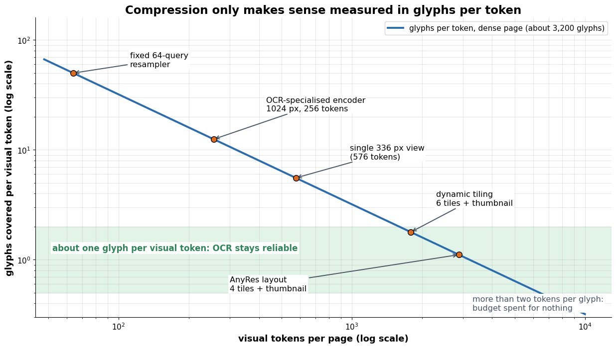
$G$ is the glyph count on the page and $c$ the glyphs per visual token; $c \approx 1$ is the practical safety line for character-accurate reading.
$N_t$ is the text prompt length and $d$ the model width, so prefill is quadratic in the combined sequence while the KV cache grows linearly.

Worked Example, One Dense A4 Page At 150 DPI:
$N_v = 4 \times 576 + 576 = 2880$
$c = 3200 / 2880 \approx 1.1$
$c = 3200 / 576 \approx 5.6$
$(2880 / 576)^2 = 25$

Assuming about 3,200 glyphs on the page, an AnyRes layout of four 336-pixel tiles plus a thumbnail lands at roughly one glyph per token, while a single 336-pixel view lands at 5.6 and reads only headlines. The last line is the bill: those extra tokens cost 25 times the attention work in prefill, which is precisely why the compressor exists and why the interesting engineering is choosing the smallest $N_v$ that still keeps $c$ near 1 for the document class you serve.

Figure 2: Compression is only meaningful relative to glyph density. Configurations inside the band give each visual token roughly one character and read reliably; a 64-slot resampler asks one token to encode about 50 glyphs. Systems trained specifically for optical text compression can operate right of the band, but at a measured precision cost, and below the band extra tokens buy nothing.

Property	Spatial channel merge	Fixed-query resampler	In-LLM pruning or merging
Mechanism	Pixel unshuffle or strided conv over the patch grid, then a linear projection	Cross-attention from K learned queries into all patch embeddings	Rank tokens by attention received in an early layer, drop or merge the tail
Budget vs resolution	Grows linearly with pixels, fixed ratio of 4x or 16x	Constant at K (typically 32 to 256) whatever the input size	Grows with pixels, then cut by a fixed keep-rate
Spatial index kept	Yes, one token maps to one known rectangle	No, slots are content-addressed and order must be relearned	Yes for survivors, but dropped regions leave holes
Training cost	One small projection, trained with the connector	A full extra transformer stage plus alignment pretraining	Usually training-free, applied at inference
Dominant failure	Long context and quadratic prefill on multi-page inputs	Reading order and rare glyphs collapse on dense pages	Whole text lines vanish when the query is not yet visible to the scorer

August 18, 2026

DL0140 Temporal Visual Grounding

What are the challenges of temporal visual grounding (predicting the start and end timestamps of a language query inside a long, untrimmed video, as in video search features built on models like InternVideo2 or TimeChat)?

Answer

Temporal visual grounding (also called temporal sentence grounding or moment retrieval) maps one natural-language query onto a single interval $(s, e)$ inside an untrimmed video, and almost every difficulty follows from one mismatch: the metric is far more precise than the signal you can afford to look at. Benchmarks report R@1 at IoU 0.7 against a human-drawn span, yet the target moment is often a few percent of a video that runs for minutes, its boundaries are genuinely ambiguous (annotators disagree by seconds about when “opens the fridge” starts), supervision is a single positive span among thousands of candidate windows, and compute forces you to subsample frames so hard that the achievable temporal resolution can be coarser than the tolerance the metric grants. Worse, the standard datasets carry strong temporal location priors, so a model that never looks at the video can score respectably and mask the fact that no grounding is happening at all. Cross-modal features add their own problem, because image-level encoders describe objects well and describe verbs, ordering, and completion poorly, which is exactly the information a query like “right after he sits down” depends on.

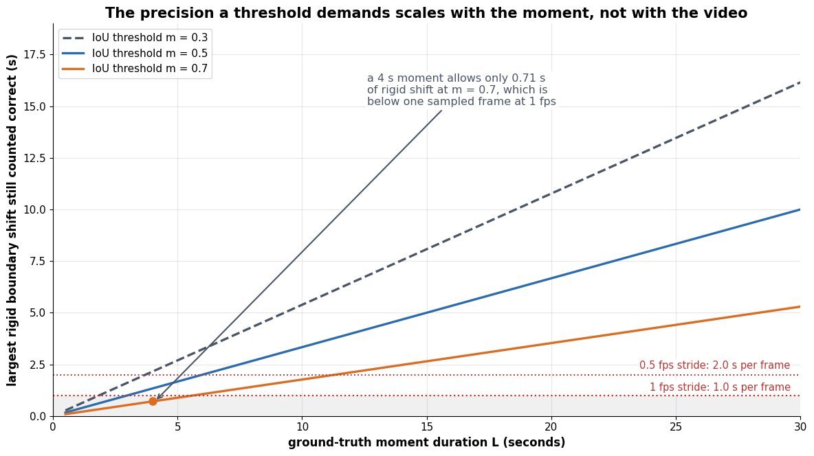
(1) Tolerance Scales With The Moment, Not The Video: at $m = 0.7$ a correctly sized 4-second moment tolerates a rigid boundary shift of only 0.71 s, so short moments demand sub-second precision while long ones are almost free.
(2) Boundary Ambiguity Lives In The Labels: event onsets and offsets are not crisp, so inter-annotator IoU sits well below 1.0 and an L1 boundary regression fits annotation noise past a certain accuracy.
(3) Sampling Stride Trades Precision Against Cost: sampling at $f$ fps sets a hard error floor near $1/(2f)$ seconds, but keeping $f$ high makes $N = fT$ large and early cross-modal fusion costs $O(N^2)$ .
(4) Features Are Weak On Temporal Semantics: frozen CLIP-style per-frame embeddings encode appearance, so verbs, order, and “before/after” relations are nearly invisible without motion-aware or video-pretrained features.
(5) Location Priors Let Blind Models Win: on Charades-STA and ActivityNet Captions the ground-truth spans cluster in predictable places, so query-only or prior-only baselines are competitive and out-of-distribution splits expose the gap.
(6) Supervision Is Sparse And Assumes One Span: a single positive interval creates extreme foreground/background imbalance, and queries matching several disjoint intervals or none at all break single-span heads outright.

Line chart of the largest rigid boundary shift still counted correct versus ground-truth moment duration, for IoU thresholds 0.3, 0.5 and 0.7, with dotted horizontal lines marking the resolution floors of 1 fps and 0.5 fps sampling; short moments at threshold 0.7 fall below the 1 fps floor

Figure 1: The tolerance the metric grants is proportional to the moment duration, so a strict threshold on short moments asks for a precision that the frame sampling stride cannot deliver. Below the dotted lines, the demanded accuracy is finer than one sampled frame, and no amount of head tuning recovers it.

Mathematical Formulation:
$I = \max(0,\ \min(\hat{e}, e) - \max(\hat{s}, s))$
$U = \max(\hat{e}, e) - \min(\hat{s}, s)$
$\mathrm{IoU} = I / U$
$\delta \leq \frac{1 - m}{1 + m}\, L$
$\mathrm{Acc}_{m} = \frac{1}{Q} \sum_{q=1}^{Q} \mathbf{1}[\mathrm{IoU}_{q} \geq m]$
$\mathcal{L} = \lambda_{1} \lVert \hat{b} - b \rVert_{1} + \lambda_{2} (1 - \mathrm{IoU})$
$N = f\,T$

Where:

$(s, e)$ is the annotated span and $(\hat{s}, \hat{e})$ the prediction, both in seconds; $I$ and $U$ are the 1D intersection and union, and the $\max(0, \cdot)$ handles disjoint spans.
$L = e - s$ is the ground-truth duration, $m$ the IoU threshold, and $\delta$ the largest rigid shift of both boundaries that still passes, obtained from $(L - \delta)/(L + \delta) \geq m$ .
$q \in \{1, \ldots, Q\}$ indexes queries and $\mathrm{Acc}_{m}$ is the usual R@1, IoU=m metric, a hard indicator that is flat inside the tolerance band and gives no gradient-like signal about how close a miss was.
$b = (s, e)$ normalized by video length, $\lambda_{1}$ and $\lambda_{2}$ the loss weights; the L1 term is scale-sensitive and the IoU term is scale-free, which is why both appear in DETR-style grounding heads.
$T$ is the video duration, $f$ the sampling rate, and $N$ the number of frame tokens; a 20-minute video at $f = 1$ gives $N = 1200$ , and self-attention over it costs $O(N^2)$ per query.

The design space has moved through three families and is now entering a fourth: sliding-window proposal ranking (dense candidate spans scored against the query, as in 2D-TAN), proposal-free span prediction (per-frame start and end distributions, as in VSLNet), DETR-style set prediction (learnable moment queries plus Hungarian matching with an L1 and IoU loss, as in Moment-DETR and CG-DETR), and video LLMs that emit timestamps as text or as dedicated time tokens. Each family inherits the same structural problems in a different shape: proposal methods make the imbalance explicit and cap resolution at the window grid, span prediction is cheap but assumes exactly one contiguous answer, set prediction handles multiple moments and a no-moment class but needs enough data to learn the matching, and LLM-based grounders quantize time into a token vocabulary and therefore trade fine boundary precision for reasoning ability. Scaling to hour-long input is a separate axis, because early fusion concatenates query and video tokens and blows up memory with $N$ , while late fusion keeps the video encoding query-independent so features can be cached and reused across thousands of queries.

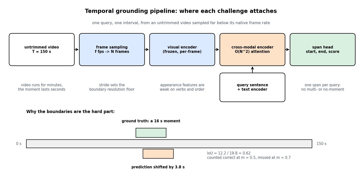
Pipeline diagram of a temporal grounding model: untrimmed video, frame sampling at f fps, frozen per-frame visual encoder, cross-modal encoder with quadratic attention, and a span head emitting start, end and score, with the query sentence and text encoder feeding into the cross-modal stage; a challenge callout sits under each stage, and a bottom timeline compares a ground-truth 16 second moment against a prediction shifted by 3.8 seconds giving IoU 0.62

Figure 2: Each pipeline stage contributes its own failure mode: the sampling stride fixes the resolution floor, the frozen per-frame encoder discards motion and ordering, early fusion makes cost quadratic in frame count, and a single-span head cannot express multiple or absent moments. The bottom timeline shows why the threshold choice dominates reported numbers: the same prediction passes at $m = 0.5$ and fails at $m = 0.7$ .

Property	Charades-STA	ActivityNet Captions	QVHighlights	MAD
Typical video length	about 30 s	about 120 s	150 s clips	full movies, about 110 min
Typical moment length	about 8 s	about 36 s	tens of seconds	about 4 s
Moment share of video	roughly a quarter	roughly a third	small but non-trivial	well under 0.1 percent
Moments per query	one	one	often several disjoint	one
Dominant difficulty	strong location prior, blind baselines score well	long vague spans, annotation bias	set prediction plus saliency, no-moment cases	extreme needle in a haystack, memory and caching

August 17, 2026

DL0139 Multi-Camera Video VLM

How do multi-camera video VLMs fuse visual inputs across asynchronous camera feeds with overlapping fields of view, as in Waymo’s surround-camera perception stack?

Answer

Fusion is three separate problems solved in a fixed order: time alignment, per-view encoding, then spatial merging. Production rigs first put every camera on one clock (PTP or GPS-locked triggers) and stamp each frame with its own capture time, because software receive time is meaningless at 30 fps. Each view is then encoded independently by a weight-shared ViT and compressed to a small token set per frame, since the raw budget is multiplicative: 6 cameras at 8 frames of 256 tokens each is $12{,}288$ visual tokens before a single word of the prompt. The merge itself comes in two families. Token-level fusion concatenates all view tokens into one LLM context and tags each token with a camera-identity, extrinsic-pose, and timestamp embedding, letting attention discover the cross-view correspondence itself; this is the route taken by surround-view multimodal models such as Waymo’s EMMA. Geometric fusion instead defines 3D query points (BEV cells or object queries), projects each one into every camera using calibrated intrinsics and extrinsics warped by ego motion to a common query time, and merges the sampled features with per-camera weights, so a point seen by two overlapping cameras is fused once rather than described twice.

(1) One Clock Before Anything Else: hardware-triggered PTP or GPS sync plus a per-frame capture timestamp is the prerequisite; without it every downstream geometric step inherits an unknown offset.
(2) Shared Encoder Per View: one ViT with tied weights runs on all $N$ views, followed by token reduction (pooling, a Q-Former, or a perceiver resampler) to keep the context finite.
(3) Token-Level Fusion Is Implicit: concatenate everything and add camera-ID, pose, and time embeddings; flexible and calibration-tolerant, but the model must learn that two tokens describe the same object.
(4) Geometric Fusion Is Explicit: project each 3D query point into every camera and merge samples with confidence weights, which deduplicates the overlap region by construction.
(5) Asynchrony Is A Pose Problem: each view is warped by the ego transform between its own capture time and the query time $t_q$ , so odometry or IMU quality bounds fusion accuracy.
(6) Token Budget Dominates Cost: tokens grow as $N \cdot T \cdot P$ while self-attention grows as $O(L^2)$ , so doubling the camera count quadruples attention FLOPs.
(7) Overlap Weighting Prevents Double Counting: weights derived from depth uncertainty and viewing angle favor the near, front-facing view over the oblique one.

The choice between the two families is not stylistic. Geometric fusion needs metric extrinsics, reasonable depth, and a rigid rig, and in exchange it gives a metrically consistent scene where 3D detection, tracking, and occupancy prediction are natural. Token-level fusion needs almost nothing beyond a camera index, survives loose or drifting calibration, and keeps the full appearance detail that a projection into a coarse BEV grid throws away, which matters for open-ended questions such as reading a sign visible in only one view. Most deployed stacks are hybrid: encode per view, warp features to a common timebase, lift to a shared 3D representation for the geometric heads, and pass a reduced token set of the same features into the language decoder for reasoning.

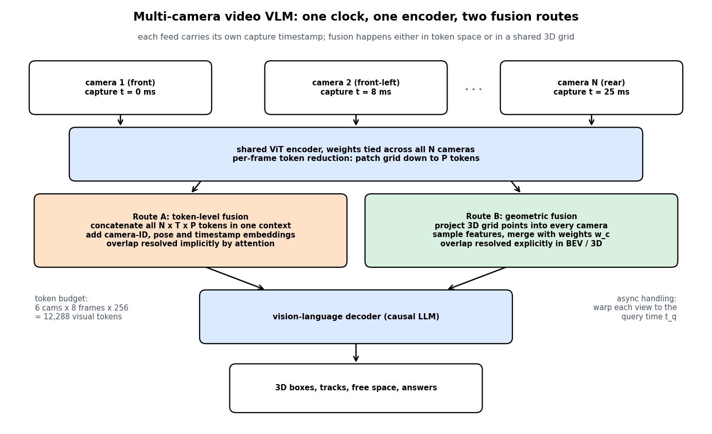
Top-to-bottom architecture diagram: three asynchronous camera feeds with different capture timestamps feed a shared ViT encoder with per-frame token reduction, which then branches into two fusion routes, token-level concatenation with camera-ID and pose embeddings on the left and geometric lifting into a shared BEV grid on the right, both feeding a vision-language decoder that emits text output

Figure 1: The pipeline is shared up to the fusion point: timestamped feeds → weight-tied ViT → token reduction, then either Route A (concatenate all tokens and let attention resolve the overlap) or Route B (project a 3D grid into every camera and merge with weights). Route A pays in context length, Route B pays in calibration and depth accuracy.

Mathematical Formulation:
$L_{vis} = N \cdot T \cdot P = 6 \cdot 8 \cdot 256 = 12288$
$\hat{X}_c = T_{c \leftarrow e}\, \Delta T(t_q, t_c)\, X_p$
$u_c = \pi(K_c\, \hat{X}_c)$
$B(p) = \frac{\sum_c m_c w_c\, F_c(u_c)}{\epsilon + \sum_c m_c w_c}$
$\Delta d = v\, |t_c - t_q|$
$\Delta d = 16.7 \cdot 0.025 = 0.42\ \text{m}$

Where:

$L_{vis}$ is the visual token count entering the decoder, with $N$ cameras, $T$ frames kept per camera, and $P$ tokens per frame after reduction.
$X_p$ is a 3D query point in the ego frame (a BEV cell center or a learned object query) and $\hat{X}_c$ is the same point expressed in camera $c$ ‘s frame at that camera’s own capture time.
$T_{c \leftarrow e}$ is the fixed extrinsic from ego to camera $c$ , and $\Delta T(t_q, t_c)$ is the ego-motion transform from the query time to the capture time, obtained from wheel odometry, IMU, or visual odometry.
$K_c$ is the intrinsic matrix, $\pi$ the perspective projection, $u_c$ the resulting pixel location, and $F_c(u_c)$ the encoder feature sampled there by bilinear interpolation.
$m_c \in \{0,1\}$ is the visibility mask (point inside the frustum and unoccluded), $w_c$ the per-camera confidence weight from depth uncertainty and incidence angle, and $\epsilon$ a guard so uncovered cells stay zero instead of dividing by zero.
$v$ is ego speed and $|t_c - t_q|$ the timestamp offset, so $\Delta d$ is the spatial error incurred by ignoring compensation; the numeric line uses $v = 16.7$ m/s (60 km/h) and a 25 ms offset expressed in seconds.

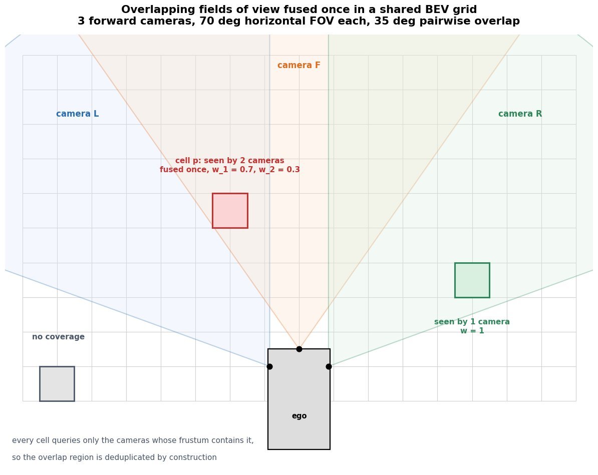
Top-down BEV diagram of an ego vehicle with three forward camera frustums drawn as shaded wedges that overlap pairwise, laid over a square BEV grid; one highlighted cell falls inside two wedges and is labeled as fused with two weights, another cell falls inside one wedge only, and a cell at the far left falls outside all wedges and is labeled as having no coverage

Figure 2: Why geometric fusion handles overlap cleanly. Each BEV cell queries every camera whose frustum contains it, so a cell in the pairwise overlap receives two samples that are averaged with confidence weights instead of appearing as two separate objects. Cells outside every frustum stay explicitly empty, which token-level concatenation cannot represent.

Asynchrony bites hardest at the selection step. With free-running 30 fps sensors, the newest available frame from each camera can be up to one full period old, so a naive “latest frame per camera” gather can mix captures spread across 33 ms. At 60 km/h the rig moves 0.55 m in that window, which is larger than the BEV cell size most stacks use, and the symptom is a smeared or duplicated object in the overlap region rather than an obvious crash. Two fixes are standard: warp features per view with $\Delta T(t_q, t_c)$ before sampling, and feed the residual offset to the model as a timestamp embedding so it can learn how much to trust a stale view. Hardware-triggered synchronous shutters remove the problem at the source and are worth the wiring cost on any rig that must produce metric output.

Left panel: timeline of four free-running 30 fps camera feeds with staggered capture phases, showing the newest frame available before a query time of 40 milliseconds for each camera and a double-headed arrow marking a 25 millisecond spread. Right panel: line chart of ego displacement in meters versus timestamp offset from 0 to 50 milliseconds for speeds of 10, 30, 60 and 100 kilometres per hour, with a dotted horizontal line at a 0.3 metre fusion tolerance

Figure 3: Free-running feeds mean the frames you gather at $t_q$ can span nearly a full frame period (left), and that spread converts directly into ego displacement (right). At highway speed even a 20 ms offset exceeds a typical 0.3 m fusion tolerance, which is why the ego-motion warp is not optional.

Property	Token-level concatenation	Dense BEV lifting	Sparse 3D queries
Shared representation	The LLM context itself, with camera-ID, pose and time embeddings	A metric BEV or voxel grid in the ego frame	A few hundred learned 3D queries with reference points
Overlap handling	Implicit; attention must learn that two tokens are one object	Explicit; one cell averages all cameras that see it	Explicit; one query attends to all views that contain its point
Asynchrony handling	Timestamp embedding only; residual error stays in the features	Ego-motion warp per view before sampling	Query propagation across frames with a motion-compensated pose
Calibration requirement	Low; a camera index and rough pose are enough	High; extrinsic drift of a degree visibly smears the grid	High for the projection, but errors stay local to each query
Cost scaling	Quadratic in N x T x P through self-attention	Linear in cameras, but grid resolution cubed in 3D	Linear in queries times cameras, cheapest at high N
Best for	Open-ended VQA, captioning, uncalibrated or ad hoc rigs	Occupancy, map and free-space prediction on a rigid rig	Streaming 3D detection and tracking under a latency budget

August 17, 2026

DL0138 Point-Informed Region VLM

Explain how Point-Informed or Region-Based Vision-Language Models incorporate bounding boxes or visual prompts directly into self-attention, as in Ferret and Molmo.

Answer

A region-based VLM has to turn a geometric object (a box, a point, a scribble) into something a transformer can consume, and there are only three places to put it: the token sequence, the positional encoding, or the attention logits. The cheapest route serializes the geometry as coordinate tokens, either quantized bins added to the vocabulary (Kosmos-2 uses 1024 location tokens over a 32×32 grid, written like <loc_0512>) or plain digit strings (Shikra), so the box reaches self-attention as ordinary keys and values with zero architecture change. The second route extracts region features with RoIAlign or a learned sampler and projects them into the language model’s embedding space as extra tokens interleaved into the prompt (GPT4RoI, Ferret), which every text token can attend to like a word. The third route never adds tokens at all: it adds a bias matrix $B$ to $QK^{\top}$ before the softmax, so patches inside the referred region get a boost and patches outside get suppressed or hard-masked to $-\infty$ . A fourth, architecture-free trick draws the prompt in pixel space (ViP-LLaVA’s overlaid arrows and circles, Set-of-Mark’s numbered masks) and lets the vision encoder’s own self-attention pick it up, which is the only option when the model is a frozen API. The choice is a trade among spatial precision, sequence growth, and how much grounding supervision you can afford to train on.

(1) Three Injection Points: geometry enters as tokens, as positional/coordinate embeddings, or as an additive term inside the attention logits, and most systems combine at least two.
(2) Coordinate Tokens Are Free But Quantized: a 1000-bin normalized grid on a 1024 px image gives roughly 1 px resolution, but the same bins on a 4K crop after tiling lose fidelity and shift under aspect-ratio padding.
(3) Region Tokens Buy Content, Not Just Location: a pooled RoIAlign vector carries appearance of the referent, so the model can describe a region it could not have isolated from coordinates alone.
(4) Attention Bias Adds Zero Parameters: $B_{ij}$ is added elementwise to the pre-softmax scores, leaving the $O(N^2 d)$ cost and the KV cache unchanged, and a per-head $\lambda_h$ can be learned.
(5) Hard Masks Destroy Context: setting $B_{ij} = -\infty$ outside the region removes exactly the surrounding evidence that relational questions need, and a fully masked row produces a degenerate softmax.
(6) Points Are Cheaper Supervision Than Boxes: Molmo’s pointing data shows a single $(x, y)$ pair is enough for counting and referring, and it avoids the box-regression ambiguity for deformable objects.
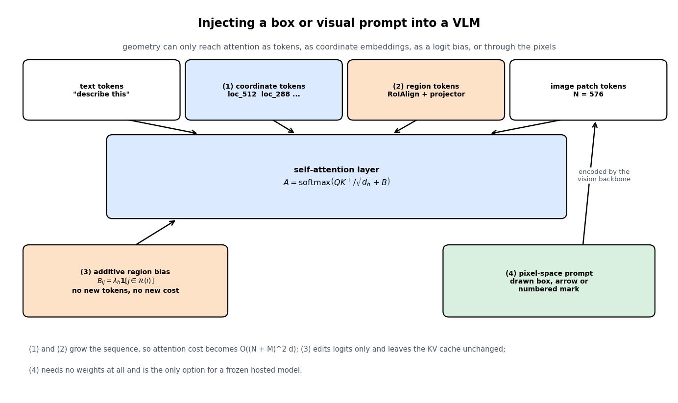
(7) Pixel-Space Prompts Work On Frozen Models: drawing the mark changes the image, not the architecture, but it occludes content and fails on thin or tiny structures.

Diagram of a vision-language model token sequence containing text tokens, quantized coordinate tokens, projected region-feature tokens and image patch tokens, all feeding a self-attention block whose pre-softmax logits receive an additive region bias matrix from the side, with a separate pixel-space visual prompt path feeding the patch tokens

Figure 1: Four ways a box reaches attention. Mechanisms (1) and (2) extend the token sequence so geometry becomes ordinary keys and values, mechanism (3) leaves the sequence untouched and edits the pre-softmax logits, and mechanism (4) modifies the pixels so the vision encoder does the work. Only (3) avoids sequence growth entirely.

The region-feature path is the one that most resembles classical detection heads: pool the backbone feature map over the box (RoIAlign → linear projector → language-model token), then concatenate a coordinate embedding so the model knows where the appearance came from, not only what it looks like. Ferret generalizes this with a spatial-aware visual sampler that samples and pools features inside an arbitrary free-form shape, so a point, a box, and a scribble all reduce to the same fixed-size token, and Groma pushes localization into the tokenizer itself by proposing regions up front and giving each one a referable ID token. The attention-bias path is complementary and is the literal reading of the question: because the softmax is invariant to nothing but its own inputs, a single additive term reweights how much probability mass a text query spends on patches inside versus outside the referent, and a moderate $\lambda_h$ concentrates mass without deleting surrounding context. In practice, training matters more than the plumbing: none of these mechanisms produces reliable grounding without a large corpus of region-text pairs, which is why grounded VLMs are trained on visual genome, RefCOCO-style referring expressions, and synthetically generated region captions.

Mathematical Formulation:
$e_r = W_v\, \mathrm{RoIAlign}(F, b) + W_c\, \psi(b)$
$\psi(b) = [\, x_1,\, y_1,\, x_2,\, y_2 \,] / S$
$Z^{(0)} = [\, E_{txt};\; e_r;\; E_{img} \,]$
$A = \mathrm{softmax}\!\left( \frac{QK^{\top}}{\sqrt{d_h}} + B \right)$
$B_{ij} = \lambda_h \, \mathbf{1}[\, j \in \mathcal{R}(i) \,]$
$\mathrm{cost} = O\big( (N + M)^2 d \big)$

Where:

$e_r$ is the region token appended to the prompt, and $Z^{(0)}$ is the full input sequence of text, region, and image-patch embeddings.
$F$ is the vision-encoder feature map, $b = (x_1, y_1, x_2, y_2)$ the box in pixels, $S$ the image side used for normalization, and $\psi(b)$ the normalized coordinate vector.
$W_v$ projects the pooled region feature into the language-model width and $W_c$ embeds the coordinates; both are the only new parameters this path needs.
$Q, K$ are the query and key projections of $Z$ , $d_h$ the per-head dimension, and $A$ the attention matrix over all $N + M$ positions.
$B$ is the additive region bias, $\mathcal{R}(i)$ the set of positions that query $i$ is encouraged to attend to (the patches overlapping the referred box), and $\lambda_h \geq 0$ the per-head bias strength; $\lambda_h = 0$ recovers plain attention and $\lambda_h \to \infty$ gives a hard mask.
$N$ is the number of visual plus text tokens, $M$ the number of added region or coordinate tokens, and $d$ the model width, so token-based injection is quadratic in $M$ while the bias term is free.

Three grayscale heatmaps of a text query's attention over an eight by eight patch grid, with a blue rectangle marking the referred region: the first with no bias shows diffuse mass spread across the image, the second with a soft additive bias concentrates mass inside the rectangle while keeping some outside, and the third with hard masking puts all mass inside the rectangle and exactly zero outside

Figure 2: The same query, the same keys, three values of $\lambda_h$ . A soft bias raises in-region mass from a small baseline to the majority while preserving outside context, which is what relational questions need; hard masking reaches 100% in-region mass and throws that context away.

Property	Coordinate tokens	Region-feature tokens	Attention bias / mask	Pixel-space prompt
Path into attention	New vocabulary or digit tokens as keys/values	Pooled RoI feature projected to an embedding	Added to pre-softmax logits	Altered patch embeddings
New parameters	Embedding rows only	Sampler plus two projections	None, or one scalar per head	None
Sequence growth	4 to 8 tokens per box	1 to 49 tokens per region	Zero	Zero
Precision limit	Bin width and tiling frame	RoIAlign grid and patch stride	Patch stride (14 or 16 px)	Stroke width and image resolution
Main failure mode	Coordinate frame drift after padding or crops	Token blowup with many regions	Loses outside context; needs a region per query	Occludes the referent; fails on small objects
Representative systems	Pix2Seq, Kosmos-2, Shikra, Qwen2.5-VL	GPT4RoI, Ferret, Groma	Region-conditioned decoders, SAM-style prompting	ViP-LLaVA, Set-of-Mark

August 17, 2026