Tag: VLM

Vision-Language Models (multimodal understanding)

DL0137 Early vs Late Fusion Multimodal

Compare Early Fusion vs. Late Fusion in multimodal models. What are the scaling limitations of early fusion architectures when scaling parameters past 100B?

Answer

The two designs differ in where the modalities meet. Late fusion (the modular VLM recipe behind BLIP-2, LLaVA, and Qwen2-VL) keeps a separately pretrained vision encoder, compresses its output through a small connector (an MLP projector, a Q-Former, or gated cross-attention), and feeds the resulting soft tokens into a pretrained text LLM, so nearly all capacity is inherited and only the connector plus a light fine-tune is trained. Early fusion (native multimodal, as in Fuyu-8B, Chameleon, and Llama 4) discretizes or linearly projects raw patches into the same token stream as text and runs one shared transformer from layer 0, so every layer attends across modalities and the model can emit image tokens as well as text. Early fusion is representationally stronger and, per recent scaling-law work, not worse per FLOP, so its problems past 100B parameters are systems and data problems rather than a representational ceiling. You cannot reuse a trained text-only 100B checkpoint, a Chinchilla-scale run now wants roughly 2T interleaved tokens that do not exist at text quality, the shared dense weights must be split between modalities, and every image inflates the sequence that attention pays $O(T^2)$ for.

(1) Meeting Point Defines The Family: late fusion joins modalities after a frozen encoder has already compressed the image; early fusion joins them at the token level, before any transformer layer.
(2) Checkpoint Reuse Is The Real Asymmetry: late fusion amortizes the trillions of text tokens already spent on the LLM, while a native 100B model pays that bill again on scarcer interleaved data.
(3) Modality Competition In Shared Weights: a dense early-fusion stack allocates the same parameters to pixels and text, so raising the image-token fraction $r$ costs text-benchmark quality and turns $r$ into a hyperparameter you cannot sweep cheaply at 100B.
(4) Token Budget Dominates The Context: one 512px image is about 1024 VQ tokens, so a four-image document spends 4096 tokens on pixels and quadratic attention absorbs the difference.
(5) Optimization Instability Grows With Width: heterogeneous token statistics drive logit growth and loss spikes, which is why Chameleon needed QK-Norm, reordered normalization, and dropout to keep a 34B run stable.
(6) Modularity Versus Capability: late fusion lets you swap the encoder or raise resolution for the price of a connector re-train, while early fusion buys interleaved any-to-any generation that a frozen tower cannot express.

Two-panel architecture diagram: the left panel shows late fusion where an image passes through a frozen ViT encoder and a trainable projector before entering a pretrained 100B LLM alongside text tokens; the right panel shows early fusion where image patches and text are tokenized into a single interleaved stream that a shared transformer trained from scratch consumes

Figure 1: Late fusion (left) is an assembly of pretrained parts, so the trainable surface is a projector of roughly 0.02B parameters and the alignment budget is on the order of 1B image-text tokens. Early fusion (right) is one homogeneous stack from random init, which is simpler to shard but means the whole 100B must be pretrained on interleaved data.

The scaling wall past 100B is mostly arithmetic. A dense 100B model trained compute-optimally wants about 2T tokens and roughly $1.2 \times 10^{24}$ FLOPs, and in native early fusion those tokens must be interleaved image-text documents; the supply of such data at web-text quality is far smaller than the text corpus, so teams either repeat data or dilute the text share and watch reasoning benchmarks regress. Late fusion sidesteps this entirely because the expensive part is already paid: aligning a connector on a couple of billion tokens with a frozen backbone is three orders of magnitude cheaper than a from-scratch native run at the same parameter count. On top of the data problem, dense early fusion suffers capacity contention, since gradients from visual reconstruction and from language modeling compete for the same MLP weights, and sparsity is the standard fix: a mixture-of-experts stack with modality-aware routing gives each modality its own parameters while keeping active FLOPs fixed, which is why recent native models are almost always sparse. Early fusion does win on the systems side (no separate vision tower to shard, no encoder-LLM pipeline bubble, and a single tokenizer path), and it is the only option when the target task requires interleaved generation or genuinely fine-grained grounding that a pooled 576-token projection has already destroyed.

Mathematical Formulation:
$h_v = W_p\, E_v(I)$
$y = \mathrm{LLM}_{\phi}([\,h_v;\, E_t(x)\,])$
$y = T_{\theta}([\,z_1, z_2, \ldots, z_T\,])$
$C \approx 6ND$
$D \approx 20N$
$N = 10^{11} \Rightarrow C \approx 1.2 \times 10^{24}$
$T = N_{img} + N_{txt}$
$C_{attn} = \Theta(L\, T^{2}\, d)$
$D_{txt} = (1 - r)\, D$

Where:

$y$ is the generated output; the first two equations are the late-fusion path and the third is the early-fusion path, where a single stack $T_{\theta}$ consumes the whole interleaved sequence.
$I$ is the image and $x$ the text; $E_v$ is the pretrained vision encoder, $E_t$ the text embedding, and $W_p$ the connector, typically the only trained matrix during alignment.
$z_t$ for $t \in \{1,\ldots,T\}$ are the interleaved tokens, either VQ image codes or linear patch projections placed in the same sequence as text tokens.
$N$ is the parameter count, $D$ the training tokens, and $C$ the training FLOPs; $D \approx 20N$ is the Chinchilla compute-optimal ratio, which for $N = 10^{11}$ demands about 2T tokens.
$L$ is the layer count and $d$ the model width, so $C_{attn}$ shows that image tokens entering the shared stack are charged quadratically, not linearly.
$r \in [0,1]$ is the image-token fraction of the pretraining mixture, so $D_{txt}$ is the surviving text budget; at fixed $C$ , every point of $r$ is taken directly out of language modeling.

Two-panel chart: left panel is a log-log plot of training FLOPs versus parameter count comparing native early fusion trained from scratch at 120 N squared against late-fusion connector alignment at four N times two billion tokens, with the gap at one hundred billion parameters annotated; right panel is a log-scale bar chart of image tokens per image for pooled projectors, SigLIP 384, Chameleon VQ, Qwen2-VL dynamic resolution, and native 1024 pixel patches

Figure 2: Left: from-scratch native training scales as $120N^{2}$ under the compute-optimal token rule, while connector alignment scales linearly in $N$ , so the gap at 100B is roughly three orders of magnitude. Right: the number of tokens an image consumes spans about an order of magnitude across tokenizers, and in early fusion every one of those tokens enters the shared quadratic attention rather than being pooled away first.

Property	Early fusion (native)	Late fusion (modular)
Fusion point	Token level, before layer 1; all layers are cross-modal	After a pretrained encoder, via a projector or cross-attention
Trainable surface	Every parameter, from random init	Connector plus optional LLM fine-tune; encoder often frozen
Data requirement at 100B	About 2T interleaved tokens, a corpus that barely exists at text quality	Order 1B to 10B image-text pairs plus instruction data
Dominant failure mode	Modality competition for dense capacity, text regression, loss spikes	Information already discarded by the frozen encoder (OCR, small objects, counting)
Upgrade path	Resolution or tokenizer changes touch the pretraining recipe	Swap the encoder or the LLM and re-align the connector
Generation ability	Interleaved any-to-any output, since image tokens are in the vocabulary	Text out only, unless a separate image decoder is bolted on
Representative systems	Fuyu-8B, Chameleon, Transfusion, Llama 4	Flamingo, BLIP-2, LLaVA-1.5, Qwen2-VL, InternVL

August 17, 2026

DL0136 Unified Multimodal Gemini Architecture

How do unified multi-modal models such as Google’s Gemini handle simultaneous natively tokenized audio, vision, and text input streams?

Answer

A unified model does not bolt encoders onto a finished language model at inference time; it is pretrained from step zero on interleaved sequences in which every modality has already been converted into tokens that live in the same $d$ -dimensional embedding space. Text passes through a SentencePiece vocabulary, images and sampled video frames through a ViT-style patch encoder, and audio through a speech encoder in the Universal Speech Model (USM) lineage operating on 16 kHz waveforms; each front end emits discrete ids or continuous soft tokens that are projected to the model width and concatenated in timestamp order into one causal sequence. From that point there is no separate fusion module: ordinary self-attention in every layer is the fusion mechanism, so a text token attends to an audio window from second 12 and to the patch tokens of the frame shown during that second at the same cost as attending to another word. The consequences of native tokenization are therefore budgetary rather than architectural, because Gemini’s published token rates are roughly 258 tokens per image tile or sampled frame and 32 tokens per second of audio, so one hour of video with its soundtrack consumes about 1M tokens and long context stops being a feature and becomes a precondition.

(1) Native Tokenization, Not An Adapter: multimodal data is present in pretraining from the first step, so the shared representation is learned jointly rather than stitched together by a projector trained on top of two frozen towers.
(2) One Shared Embedding Space: a per-modality encoder plus a linear projection maps sub-words, patches, and audio frames into the same $\mathbb{R}^{d}$ , which is what makes concatenation legal.
(3) Self-Attention Does The Cross-Modal Work: there is no cross-attention adapter per modality, and the price is a $O(L^2 d)$ prefill over the combined length.
(4) Timestamp-Ordered Packing: tokens from the same second of an audio-visual clip are placed adjacent, so co-occurring events are a few hundred positions apart instead of hundreds of thousands.
(5) Token Rates Set The Budget: 258 tokens per frame, 32 tokens per audio second, and 1 fps frame sampling as the lossy compression knob that decides what the model can even see.
(6) The Output Side Can Be Multimodal Too: a single next-token head over a vocabulary extended with discrete image and audio codec tokens lets one decoder emit text, pixels, or speech without a separate generator.

Architecture diagram with three input lanes for text, image or video, and audio, each passing through its own tokenizer or encoder and a linear projection into a shared d-dimensional space, then merging into one interleaved token sequence in timestamp order that feeds a single decoder-only transformer with full self-attention, which emits text tokens, discrete image tokens, and audio codec tokens

Figure 1: Three front ends, one sequence, one stack. The only modality-specific parameters sit in the encoders and projections; after that the tokens are indistinguishable to the transformer, and the output modality is decided purely by which token ids the single next-token head emits.

Two design decisions do most of the work. The first is early fusion: because all three streams enter the same stack as tokens, cross-modal alignment is learned by the same attention weights that learn syntax, which is what lets the model join a spoken sentence to whatever was on screen while it was said. A late-fusion alternative, where a frozen vision tower is glued to a frozen LLM through a projector or Flamingo-style cross-attention adapter, is far cheaper to train but confines modality interaction to the adapter, while a cascade (audio → ASR → LLM → TTS) discards everything the transcript does not carry, including speaker identity, prosody, laughter, and overlapping non-speech events. The second decision is packing order. Placing the frame tokens and the audio tokens of the same second next to each other keeps relative position encodings informative and keeps local attention patterns useful, whereas a modality-blocked layout pushes a frame and its own soundtrack thousands of positions apart. Frame rate is then the compression knob: 1 fps is adequate for scene-level questions but structurally unable to represent a 200 ms gesture, a single flashed frame, or the exact moment a door closes.

Two token-sequence strips compared: the top strip alternates a wide block of 258 image tokens with a thin slice of 32 audio tokens for each of four consecutive seconds in timestamp order, and the bottom strip places all four image blocks first followed by all four audio slices, with a double-headed arrow showing that frame zero and its own audio are now 1032 tokens apart

Figure 2: The same tokens, two layouts. Time-interleaved packing keeps each frame beside the 32 audio tokens recorded during it, while modality-blocked packing separates them by 1,032 positions, which is why audio-visual grounding degrades even though attention can technically still reach across the whole sequence. The width ratio also shows the real cost structure: vision dominates the budget roughly 8 to 1 over audio.

Mathematical Formulation:
$u_i = W_m \phi_m(x_i)$
$S = (u_1, u_2, \ldots, u_L)$
$L = L_{\mathrm{txt}} + 258 N_f + 32 T_a$
$\mathrm{prefill} = O(L^2 d)$
$p(y_{1:M}) = \prod_{j=1}^{M} p(y_j \mid S, y_{1:j-1})$

Where:

$u_i \in \mathbb{R}^{d}$ is the $i$ -th token embedding in the shared space and $x_i$ the raw unit behind it (a sub-word, an image tile, or a short audio window).
$\phi_m$ is the front end for modality $m \in \{\mathrm{txt}, \mathrm{img}, \mathrm{aud}\}$ and $W_m$ its projection to the model width $d$ ; text is an embedding lookup over discrete ids, vision and audio produce continuous soft tokens.
$S$ is the single causal sequence, ordered by timestamp rather than by modality, and $L$ is its length.
$L_{\mathrm{txt}}$ is the text token count, $N_f$ the number of image tiles or sampled frames at 258 tokens each, and $T_a$ the audio duration in seconds at 32 tokens each.
The prefill term is quadratic in $L$ while the KV cache grows linearly, so audio and video inflate both compute and memory before a single output token is produced.
$y_{1:M}$ is the generated output drawn from one next-token distribution whose vocabulary may include discrete image and audio codes alongside sub-words.

Token Budget For One Hour Of Video With Sound:
$3600 \times 258 = 928800$
$3600 \times 32 = 115200$
$L = 928800 + 115200 = 1044000$

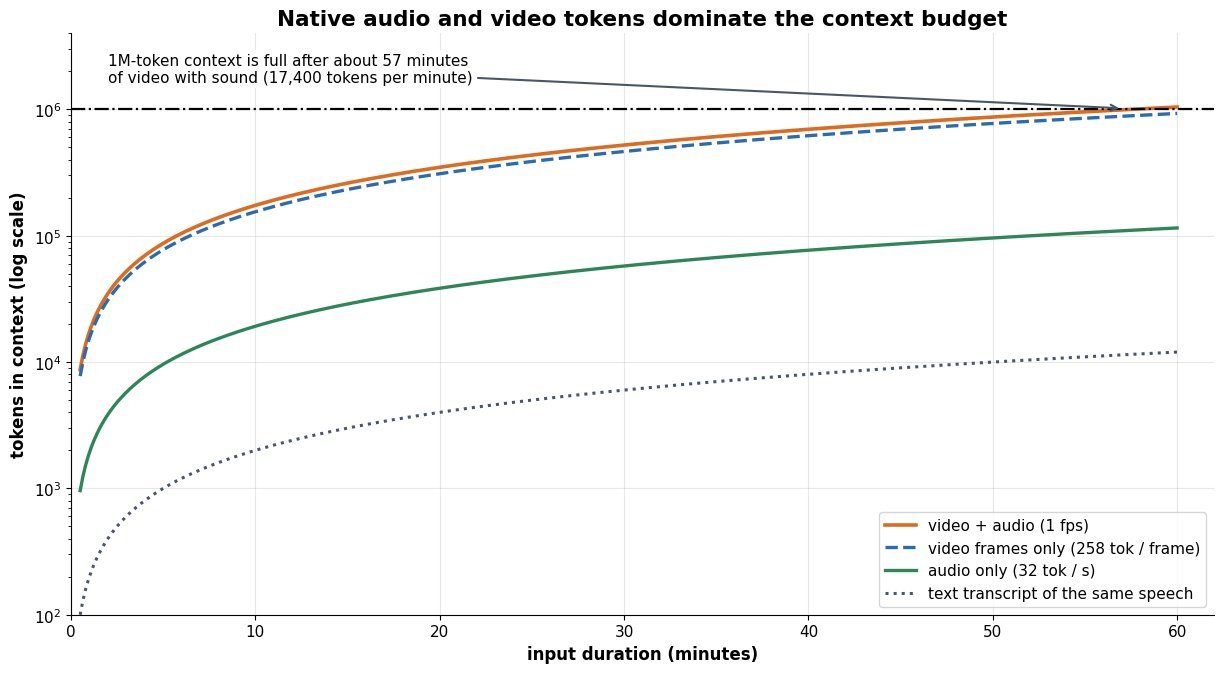
A single hour of ordinary video therefore saturates a 1M-token window, which explains why native multimodality and million-token context arrived together in Gemini 1.5 rather than as separate features. It also explains where production effort actually goes: not into inventing a fusion block, but into deciding frame rate, tile count, and audio span so that the useful evidence survives tokenization, and into paying the quadratic prefill only for the segments that matter.

Log-scale line chart of tokens consumed versus input duration in minutes for four streams: a text transcript at about 200 tokens per minute, audio only at 1920 tokens per minute, video frames only at 15480 tokens per minute, and video plus audio at 17400 tokens per minute, with a dashed horizontal line marking a one-million-token context that the video plus audio curve reaches at about 57 minutes

Figure 3: Native tokens are not cheap. At published rates, a spoken transcript costs about 200 tokens per minute while the same minute of video plus audio costs roughly 17,400, so the entire 1M-token context is spent after about 57 minutes. Every design choice about frame rate, tiling, or clip trimming is a move along this line.

Property	Text	Vision (image / video)	Audio
Front end	SentencePiece sub-word vocabulary, discrete ids	ViT-style patch encoder emitting continuous soft tokens	Speech encoder in the USM lineage over 16 kHz audio
Token rate	About 1 token per 4 characters	About 258 tokens per tile, and per sampled frame at 1 fps	32 tokens per second, independent of content
Temporal handling	Sequence order only, no clock	Frames sampled at a fixed rate and packed in timestamp order	Continuous, packed beside the frames of the same second
Native generation	Standard next-token softmax	Discrete image tokens in Gemini 2.0 native image output	Codec tokens in the native-audio and Live streaming models
Dominant failure mode	Tokenizer fragments rare words, digits, and code	1 fps sampling misses sub-second events, and tiling explodes the budget	Coarse rate blurs fine prosody, and long clips crowd out the prompt

August 17, 2026

DL0135 Dynamic High-Resolution ViT

How do Dynamic High-Resolution ViT slicing architectures handle non-standard aspect ratios and high-resolution images without spatial distortion?

Answer

A pretrained vision tower expects one fixed square input, usually $336 \times 336$ or $448 \times 448$ , with exactly one learned position embedding per patch. Squashing a $1500 \times 500$ receipt or slide into that square applies anisotropic scaling (0.30x horizontally against 0.90x vertically), which shears glyphs and bar charts before the encoder sees a single pixel, while interpolating the position-embedding grid up to native resolution is both off-distribution and quadratically expensive in attention. Dynamic high-resolution slicing, the AnyRes family used by LLaVA-NeXT, UReader, Monkey, MiniCPM-V and InternVL 1.5, avoids both by never changing the encoder’s input size: it picks a tile grid whose aspect ratio best matches the image, resizes the image to exactly $n_w S \times n_h S$ , cuts it into $n_h n_w$ native-resolution tiles that are encoded independently, and appends a downsampled full-image thumbnail to restore the global layout that slicing destroys. Because the target width and height are both integer multiples of the same tile size chosen to match the input ratio, the horizontal and vertical scale factors are (nearly) equal, so the resize is isotropic and no geometry is distorted. What remains is a budgeting problem: the token count grows linearly in tiles, so token compression and a cap $N_{\max}$ on the tile product decide how much resolution you can actually afford.

(1) Aspect-Ratio Matched Grid: enumerate all grids with $n_h n_w \leq N_{\max}$ and pick the one minimizing the log-ratio mismatch against $W/H$ , which is exactly the quantity that becomes anisotropic shear if you get it wrong.
(2) Tiles Stay At Native Resolution: every tile is precisely $S \times S$ , so the frozen CLIP or SigLIP tower runs at its pretraining resolution with no position-embedding interpolation and no distribution shift.
(3) Thumbnail Carries Global Context: tiles are encoded independently, so no attention crosses a seam; a low-resolution whole-image view is concatenated to supply page layout and object-scale cues.
(4) Linear Instead Of Quadratic Attention: encoding $K$ tiles of $M$ patches costs $K \cdot O(M^2)$ rather than $O(K^2M^2)$ for one giant grid, a $K$ -fold saving that is why slicing scales to 4K pages.
(5) Token Compression Is Mandatory: a pixel-unshuffle of stride 2 folds each $2 \times 2$ patch neighborhood into one embedding, cutting 1024 patches per 448 tile to 256 tokens; without it a 12-tile page costs over 13k tokens.
(6) The LLM Must Be Told The Layout: the flattened tile sequence is ambiguous, so implementations insert row separator tokens or 2D tile indices, otherwise a $3 \times 1$ and a $1 \times 3$ arrangement look identical downstream.

Two-panel diagram of a 1500 by 500 panoramic input containing a reference circle. The left panel resizes it into a single 448 by 448 square, where the circle becomes a narrow vertical ellipse because horizontal scale is 0.30x and vertical scale is 0.90x. The right panel matches a 3 by 1 tile grid, resizes to 1344 by 448 with both axes at 0.90x so the circle stays circular, cuts it into three native-resolution 448 tiles, and adds a low-resolution global thumbnail.

Figure 1: The reference circle is the whole story. A single square resize applies different scale factors per axis, so the circle becomes an ellipse and every glyph shears; the aspect-ratio-matched grid scales both axes by 0.90x, keeps each tile at the encoder’s native $448 \times 448$ , and pays for the lost cross-tile view with one global thumbnail.

Two details separate a correct implementation from a leaky one. First, the resize to $n_w^\ast S \times n_h^\ast S$ is only exactly isotropic when the chosen grid ratio equals the image ratio; otherwise a residual anisotropy survives, equal to the log mismatch, and it is bounded by how fine your candidate set is. With $N_{\max} = 6$ a 4:3 photo still carries 0.29 of residual log-anisotropy because the exact $3 \times 4$ grid needs 12 tiles, which is why InternVL 1.5 raises $N_{\max}$ to 12 and InternLM-XComposer2-4KHD pushes to 55 tiles, and why some systems pad to the grid instead of stretching. Second, slicing changes what the encoder can see: a table row spanning a vertical seam is split across two independently encoded tiles, so the fusion must happen inside the language model rather than in the vision tower, and this is the main reason answers to fine-grained OCR questions degrade near tile boundaries. Token cost is the binding constraint in production: LLaVA-NeXT at $S=336$ with at most 4 tiles plus a base view spends $5 \times 576 = 2880$ tokens per image, and InternVL 1.5 with 12 tiles plus a thumbnail spends $13 \times 256 = 3328$ only because pixel shuffle compresses each tile fourfold.

Mathematical Formulation:
$\mathcal{G} = \{(n_h, n_w) : n_h n_w \leq N_{\max}\}$
$(n_h^\ast, n_w^\ast) = \arg\min_{\mathcal{G}} \left| \log \frac{n_w}{n_h} - \log \frac{W}{H} \right|$
$s_x = \frac{n_w^\ast S}{W}$
$s_y = \frac{n_h^\ast S}{H}$
$D = \left| \log \frac{s_x}{s_y} \right|$
$T = (n_h^\ast n_w^\ast + 1) \frac{S^2}{p^2 r^2}$

Where:

$(n_h^\ast, n_w^\ast)$ is the selected tile grid, and $\mathcal{G}$ the candidate set of grids whose tile product stays within the budget $N_{\max}$ .
$W$ and $H$ are the original image width and height, and $S$ is the encoder’s native side length (336 for LLaVA-NeXT, 448 for InternVL 1.5).
$s_x$ and $s_y$ are the per-axis scale factors of the resize, and $D$ is the residual anisotropy: $D = 0$ means the resize is isotropic and geometry is preserved exactly.
$T$ is the vision-token count fed to the LLM, with the $+1$ accounting for the global thumbnail.
$p$ is the patch size (typically 14) and $r$ the pixel-shuffle stride, so $S=448, p=14, r=2$ gives $1024/4 = 256$ tokens per tile.
The objective is stated in log space because minimizing $|\log(n_w/n_h) - \log(W/H)|$ is identical to minimizing $D$ , which makes aspect matching and distortion control the same problem.

Two charts. Left: residual log-anisotropy versus the maximum tile product for images of aspect ratio 4:3, 3:1, 5:1 and 8:1, showing step decreases to zero when an exactly matching grid enters the candidate set, with the 4:3 curve stuck at 0.29 until twelve tiles are allowed. Right: vision-token count versus tile count for pixel-shuffle stride 1 and stride 2, with a horizontal 4096-token image budget line that stride 1 crosses at three tiles while stride 2 stays under it through twelve tiles.

Figure 2: The two knobs pull against each other. Raising $N_{\max}$ is what drives residual anisotropy to zero for awkward ratios (left), but each extra tile buys a fixed block of tokens, so only pixel-shuffle compression keeps a 12-tile page inside a realistic per-image token budget (right).

Property	Square resize + PE interpolation	Dynamic tiling (AnyRes)	Native dynamic resolution
Aspect handling	Anisotropic stretch, or padding that wastes most of the input area	Isotropic up to grid quantization; residual anisotropy shrinks as N_max grows	Exact: the patch grid itself takes the image’s shape, no quantization
Encoder reuse	Frozen tower reused, but interpolated position embeddings go off-distribution	Frozen tower reused unchanged at its exact pretraining resolution	Requires training or adapting the tower with 2D RoPE and variable-length packing
Attention cost	Quadratic in total patches once resolution is raised	Linear in tiles: K independent O(M squared) passes, easy to batch	Quadratic over the full image unless windowed or block-diagonal attention is used
Global context	Complete but low detail; small text is unrecoverable	Broken at seams; restored approximately by the thumbnail and separator tokens	Intact, every patch can attend to every other patch in the image
Representative systems	Original LLaVA, BLIP-2, early CLIP-based VLMs	UReader, Monkey, LLaVA-NeXT, MiniCPM-V, InternVL 1.5 and 2.5	NaViT, Idefics2, Qwen2-VL and Qwen2.5-VL, Pixtral

August 17, 2026

DL0134 Interleaved Vision-Language Architectures

Explain Interleaved Vision-Language Architectures. How do models pre-trained on mixed sequences of raw image tokens and text tokens differ from cross-attention models?

Answer

An interleaved vision-language architecture flattens a document into one sequence that alternates text spans and images, projects each image’s patch features into the language model’s embedding space, and trains a single decoder with ordinary next-token prediction over the mixed stream. This is early fusion: visual tokens occupy real sequence positions, so they are keys and values for every text token in every layer, and text tokens are keys and values for the image. The alternative family, cross-attention conditioning (Flamingo, Idefics1), keeps vision outside the text sequence: a frozen ViT plus a Perceiver resampler compresses each image to a fixed $R = 64$ latents, and newly inserted gated cross-attention layers let the frozen LM read those latents without ever lengthening its own sequence. The consequences are structural rather than cosmetic. Early fusion makes cost quadratic in the joint length $L = N_t + M N_v$ and demands full multimodal pre-training, but it gives uniform bidirectional-within-causal mixing, unlimited image ordering, and (with discrete VQ image tokens) the ability to generate images from the same head. Cross-attention decouples image count from the text sequence and protects a strong frozen LLM, at the price of a hand-designed conditioning path, per-image attention masks that weaken multi-image relational reasoning, and no route to image output.

(1) Where Fusion Happens: early fusion concatenates projected patch embeddings into the token stream, so mixing occurs in every self-attention layer; cross-attention confines mixing to a handful of inserted layers reading a fixed latent set.
(2) Sequence Length Is The Cost Model: a ViT-L/14 at 336 px yields $N_v = 576$ tokens per image, so eight images add 4608 positions and roughly $100\times$ the attention cost of a text-only forward pass.
(3) Attention Pattern And Multi-Image Reasoning: Flamingo masks each text token to cross-attend only to the most recent preceding image, while early fusion lets any token attend to all earlier images and their surrounding text.
(4) Parameter Budget And Text Regression: cross-attention adds new trainable blocks around a frozen LM and preserves text-only quality by construction; early fusion updates the whole backbone and risks catastrophic forgetting unless text data is replayed.
(5) Generation Symmetry: only the interleaved token-in-sequence form can emit images, because image outputs must live in the same vocabulary the head predicts (Chameleon, Emu3).
(6) Data Requirement: both families need interleaved web corpora such as M3W or OBELICS rather than caption pairs, since few-shot in-context learning is what interleaving buys.

Two-panel architecture diagram: left panel shows interleaved early fusion where text token groups and 576-token image groups alternate in one row feeding a single causal self-attention stack and a joint-vocabulary next-token head; right panel shows cross-attention conditioning where an image passes through a frozen ViT and a Perceiver resampler producing 64 latents that are read by gated cross-attention layers inserted between frozen language model blocks

Figure 1: The two conditioning paths. In early fusion the image becomes sequence positions inside the shared stack, so every layer mixes modalities and the sequence grows with each image. In cross-attention conditioning the image stays outside the text sequence as a fixed set of $R$ latents, read through gated layers whose gate starts at zero so the frozen LM is initially unchanged.

Practice has converged on early fusion, and the reason is mostly negative: the cross-attention path is an extra design surface with its own hyperparameters (how many layers to insert, resampler depth, latent count, gate schedule) and it caps the visual information at $R$ latents regardless of image resolution, which destroys dense OCR and chart reading. Ablations in MM1 found the interleaved token-in-sequence recipe matched or beat cross-attention at equal scale while being simpler, and the lineage of the same lab’s open models makes the shift explicit: Idefics1 (Flamingo-style cross-attention) → Idefics2 (early fusion with pooled visual tokens). Early fusion then imports the cross-attention family’s one real advantage, token compression, without its plumbing: Idefics3 pixel-shuffles $2 \times 2$ patch blocks into one token, Qwen2-VL merges adjacent patches in the projector, and both keep the compressed tokens in the main sequence. What remains genuinely hard in early fusion is positional encoding for a 2D object embedded in a 1D stream, handled by explicit row-separator tokens in Fuyu or by multimodal rotary embeddings that give an image token separate height, width, and time indices.

Mathematical Formulation:
$N_v = (H/P)\,(W/P)$
$L = N_t + M\,N_v$
$C_{\mathrm{self}} = O(L^2 d)$
$Z = \mathrm{Resampler}(\mathrm{ViT}(I)) \in \mathbb{R}^{R \times d}$
$C_{\mathrm{cross}} = O(N_t\, M R\, d)$
$y_\ell = h_\ell + \tanh(\alpha_\ell)\,\mathrm{XAttn}(h_\ell, Z)$

Where:

$H, W$ are the image height and width and $P$ the patch size, so $N_v$ is the visual tokens per image: at $336/14$ this is $24 \times 24 = 576$ .
$N_t$ is the number of text tokens, $M$ the number of images in the document, and $L$ the joint sequence length the early-fusion decoder actually processes; $d$ is the model width.
$C_{\mathrm{self}}$ is the self-attention cost, quadratic in $L$ , so each added image contributes both its own $N_v^2$ block and cross terms with all existing tokens.
$I$ is the raw image, $Z$ the resampled latents, and $R \ll N_v$ the latent count ( $R = 64$ in Flamingo), which is why $C_{\mathrm{cross}}$ is linear in $M$ and leaves the LM’s own $O(N_t^2 d)$ untouched.
$h_\ell$ are the frozen LM hidden states at layer $\ell$ and $\alpha_\ell$ a learned scalar gate initialized to zero, so $\tanh(\alpha_\ell) = 0$ makes the inserted block an identity at step 0 and training degrades the language model gradually rather than abruptly.

Line chart of attention cost normalized to a text-only forward pass versus the number of images from one to eight, with three curves: early fusion at 576 tokens per image rising quadratically to about one hundred times, early fusion with four-times pooling at 144 tokens per image rising to about ten times, and cross-attention with 64 latents per image rising linearly to about two times

Figure 2: Why token count dominates the choice. Early fusion pays $O(L^2)$ in the joint sequence, so eight full-resolution images cost roughly $100\times$ a text-only pass, while cross-attention stays near $2\times$ because its cost is linear in $M R$ . Patch pooling recovers most of the gap without leaving the sequence, which is the modern compromise.

Property	Interleaved early fusion	Cross-attention conditioning
Image position	Real sequence positions inside the decoder	Outside the sequence, as fixed keys and values
Cost in image count	Quadratic through the joint length L	Linear, and only in the inserted layers
Trainable surface	Projector plus the whole backbone, usually full pre-training	Resampler and gated cross-attention only, LM frozen
Visual detail ceiling	Scales with resolution; supports OCR and dense charts	Capped at R latents regardless of resolution
Multi-image reasoning	All prior images visible to every token	Typically masked to the most recent image per text token
Image generation	Possible with discrete VQ image tokens in one vocabulary	Not possible; the path is input-only
Representative models	Fuyu-8B, Chameleon, Idefics2/3, MM1, Qwen2-VL, Emu3	Flamingo, OpenFlamingo, Idefics1, Llama 3.2 Vision

August 17, 2026

DL0133 VLM Fusion: Cross-Attention, Q-Former, and MLP

Compare Cross-Attention fusion, Perceiver Resampler / Q-Former, and Linear/MLP Projection (e.g., LLaVA) for vision-language alignment.

Answer

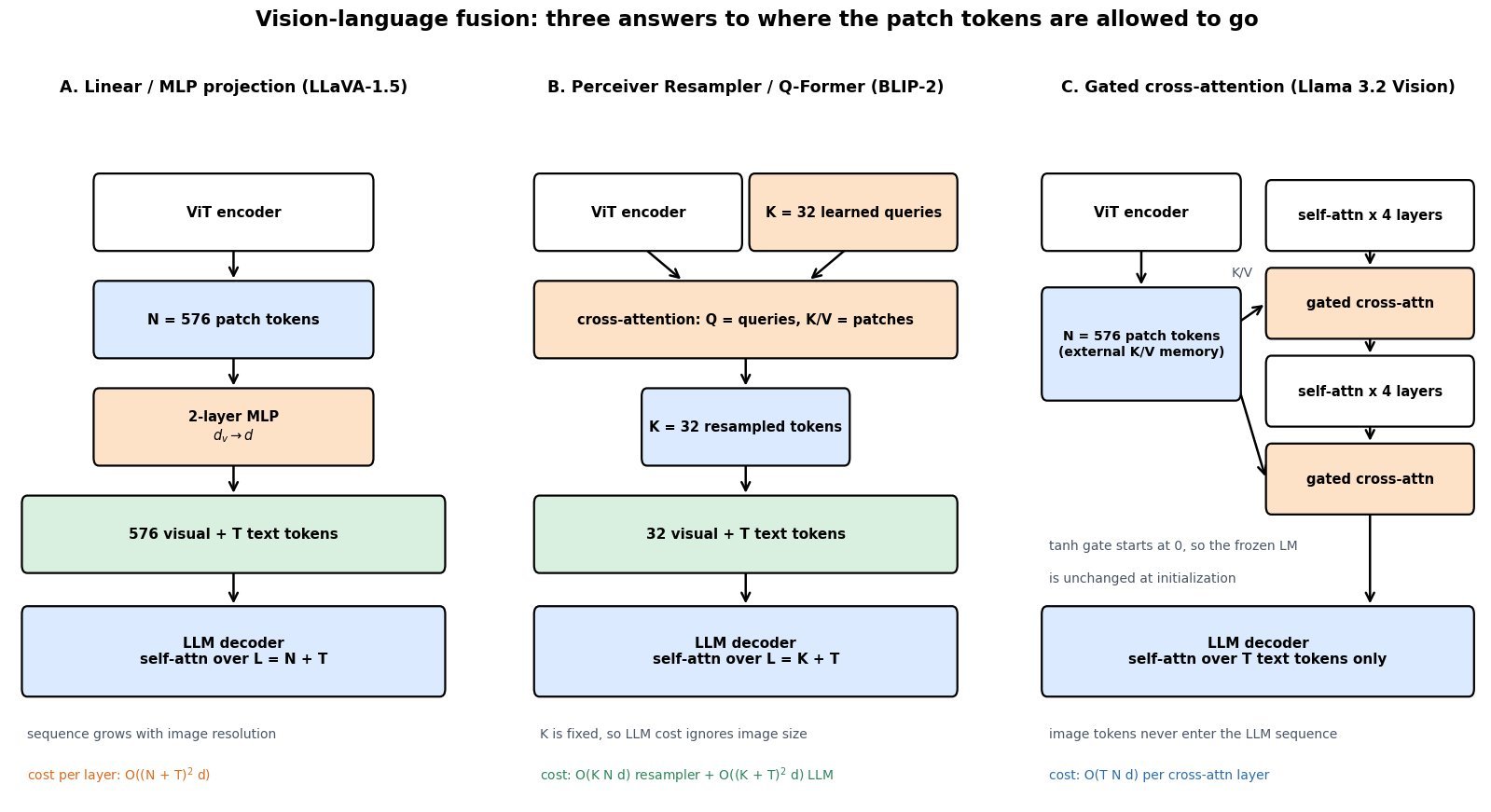
All three designs answer one question: where does the frozen vision encoder’s patch grid meet the language model? Linear/MLP projection (LLaVA, LLaVA-1.5, Qwen2-VL, InternVL) maps every patch embedding into the LLM’s token space with a two-layer MLP and concatenates the result onto the text sequence, so vision and language share one self-attention stack. Perceiver Resampler / Q-Former (Flamingo, BLIP-2) inserts a small cross-attention module in which a fixed set of $K$ learned queries (64 latents in Flamingo, 32 in BLIP-2) attends over the $N$ patch tokens and emits exactly $K$ vectors, decoupling the LLM’s sequence length from image resolution. Gated cross-attention fusion (Flamingo’s xattn-dense blocks, Llama 3’s vision adapter, NVLM-X) never puts image tokens in the LLM sequence at all: new cross-attention layers are interleaved into the language stack (every fourth layer in Llama 3) and read the patch tokens as an external key/value memory, with a tanh gate initialized to zero so the model starts out behaviorally identical to the text-only LLM. The trade-off is compute versus fidelity versus intrusiveness: MLP concatenation is the simplest and preserves the most visual detail but makes prefill grow as $O((N+T)^2)$ ; resampling is cheapest and constant-cost but imposes a hard information bottleneck; cross-attention keeps text throughput almost untouched and protects a frozen LLM, at the price of new parameters and a more complex training recipe.

(1) Where The Visual Tokens Live: MLP projection puts them inside the LLM sequence, a resampler puts a compressed $K$ of them inside, and cross-attention keeps them outside as an external memory.
(2) Prefill Cost Scaling: concatenation pays $O((N+T)^2 d)$ per layer, a resampler pays $O((K+T)^2 d)$ with $K \ll N$ , and cross-attention pays $O(T N d)$ only in the inserted layers.
(3) Added Parameters: LLaVA-1.5’s connector is roughly 20M parameters of MLP, BLIP-2’s Q-Former is about 188M with a BERT-base initialization, and Llama 3’s cross-attention adapter adds tens of billions at the 405B scale.
(4) Information Bottleneck: a fixed $K$ caps how much of a high-resolution image can survive, which is why resampler-based models underperform on dense OCR, charts, and counting.
(5) Frozen Versus Tuned Backbones: the Idefics2 ablation found cross-attention wins when the LLM is frozen, while the fully autoregressive concatenation design wins once the LLM is unfrozen.
(6) Token Count Beats Connector Design: MM1’s ablations show the connector type matters far less than image resolution and visual token count, which is why the field converged on MLP plus cheap token compression.

Three-panel architecture diagram. Panel A: ViT encoder produces 576 patch tokens, a two-layer MLP maps them into the LLM token space, and they are concatenated with T text tokens so self-attention runs over N plus T positions. Panel B: 32 learned queries cross-attend over the 576 patch tokens to produce 32 resampled tokens, which are concatenated with the text so self-attention runs over K plus T positions. Panel C: patch tokens stay outside the LLM as an external key value memory read by gated cross-attention layers inserted every fourth self-attention block, so self-attention still runs over T text tokens only.

Figure 1: The three fusion families differ only in where the patch tokens are allowed to go. Concatenation admits all $N$ of them into the shared sequence, a resampler admits a fixed $K$ , and gated cross-attention admits none, reading them instead as an external memory through layers whose tanh gate starts at zero.

The training recipe follows from the architecture. An MLP connector is so small that a two-stage schedule with about 558K caption pairs for alignment and 665K instruction samples for tuning is enough to reach state-of-the-art benchmark scores, which is what made LLaVA-1.5 reproducible on a single node. A Q-Former is a real transformer that must learn what to query, so BLIP-2 needs a dedicated representation-learning stage (contrastive, matching, and captioning objectives) before the generative stage, and remains the least data-efficient of the three per unit of final accuracy. Cross-attention sits in between: the gate makes optimization stable and lets you keep the language model frozen, so text benchmarks cannot regress, but you are training new layers that must learn to be useful without ever seeing visual tokens in the residual stream. NVLM’s controlled comparison is the cleanest evidence on the trade-off, finding the decoder-only concatenation variant stronger on OCR and multimodal reasoning while the cross-attention variant gave better throughput on high-resolution inputs.

Mathematical Formulation:
$Z = E_v(I) \in \mathbb{R}^{N \times d_v}$
$H_v = W_2\,\sigma(W_1 Z) \in \mathbb{R}^{N \times d}$
$L = N + T$
$R = \mathrm{Attn}(Q, Z, Z) \in \mathbb{R}^{K \times d}$
$H_t \leftarrow H_t + \tanh(\alpha)\,\mathrm{Attn}(H_t, Z, Z)$
$C_{\mathrm{self}} = O(L^2 d)$
$C_{\mathrm{cross}} = O(T N d)$

Where:

$I$ is the input image, $E_v$ the vision encoder (typically a frozen CLIP or SigLIP ViT), and $Z$ its patch token grid.
$H_v$ is the projected visual sequence, with $W_1, W_2$ the connector weights and $\sigma$ a GELU nonlinearity; a single $W$ recovers the original linear projection of LLaVA-1.
$N$ is the patch count ( $576$ for ViT-L/14 at 336 px), $T$ the text length, $L$ the LLM sequence length, $d$ the LLM width, and $d_v$ the vision width.
$Q \in \mathbb{R}^{K \times d}$ are the learned latent queries and $R$ the resampled output; $K$ is fixed at design time, so $R$ has the same size for a thumbnail and for a 4K page.
$H_t$ is the text hidden state inside the LLM and $\alpha$ the scalar gate parameter, initialized so that $\tanh(\alpha) = 0$ and the pretrained language behavior is exactly preserved at step zero.
$C_{\mathrm{self}}$ is the per-layer self-attention cost that concatenation inflates, and $C_{\mathrm{cross}}$ the per-layer cost of a cross-attention block, which is linear in $N$ rather than quadratic.

Log-scale line chart of relative prefill attention cost versus number of visual tokens from zero to 2880, for a 512-token text prompt and a 32-layer language model. The MLP concatenation curve rises quadratically to about forty-four times the text-only baseline, the gated cross-attention curve rises linearly to about two point four times, and the 64-latent resampler curve stays nearly flat at about one point four times.

Figure 2: Prefill attention cost relative to a text-only forward pass at $T = 512$ . At $2880$ visual tokens, concatenation costs about $44\times$ the text-only baseline because the whole stack pays $O((N+T)^2)$ , gated cross-attention costs about $2.4\times$ since only 8 of 32 layers see the image and they scale as $O(TN)$ , and a 64-latent resampler stays near $1.4\times$ because the LLM never sees more than $K + T$ positions.

Property	Linear / MLP projection	Perceiver Resampler / Q-Former	Gated cross-attention
Tokens entering the LLM sequence	All N patch tokens (576 at 336 px, thousands with tiling)	Exactly K latents (32 in BLIP-2, 64 in Flamingo)	None; patch tokens are external keys and values
Prefill scaling in image size	Quadratic, O((N+T)^2 d) in every layer	Constant for the LLM, linear O(KN d) in the resampler	Linear, O(TN d) in the inserted layers only
Added parameters	Smallest; a 2-layer GELU MLP, roughly 20M	Medium; about 188M for the BERT-base Q-Former	Largest; new attention plus FFN blocks scaled to the LLM width
Training complexity	Lowest; align then instruction-tune on about 1.2M samples	Highest; needs a separate representation-learning stage to converge	Moderate; the zero-init tanh gate makes the warm start stable
Effect on a frozen LLM	Weakest option when frozen; usually the LLM must be tuned	Works frozen, which is exactly why BLIP-2 used it	Best; text-only behavior is provably unchanged at initialization
Main weakness	Context blowup with high resolution, video, or many images	Fixed-K information bottleneck hurts OCR, charts, and counting	Extra parameters and weaker reported OCR and reasoning transfer
Representative models	LLaVA, LLaVA-1.5, Qwen2-VL, InternVL, NVLM-D	Flamingo resampler, BLIP-2, InstructBLIP, Idefics	Flamingo xattn-dense, Llama 3.2 Vision, NVLM-X

August 17, 2026

DL0116 Video VLM Temporal Sampling

How do video VLMs balance temporal sampling resolution against KV cache memory limits when processing multi-hour video streams, as in Google’s Gemini video understanding?

Answer

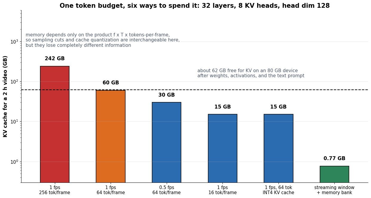
A video VLM has no separate temporal-resolution dial: it flattens the stream into one token sequence, so frame rate, tokens per frame, and clip length all collapse into a single token count $N = f \cdot T \cdot t_f$ , and that count fixes both the KV cache size (linear in $N$ ) and the prefill cost (quadratic in $N$ ). Two hours sampled at 1 fps with 64 tokens per frame is 460,800 tokens; on a Llama-3-8B-class decoder with 32 layers, 8 KV heads of head dimension 128, and a bf16 cache, each token costs 128 KB of KV, so the cache alone is roughly 60 GB, against the roughly 62 GB an 80 GB H100 has free after weights and activations. Multiply the frame rate by four or keep the encoder’s full 256 tokens per frame and you are at 240 GB, which no single device holds. Production systems therefore invert the question: fix a token budget from the memory and latency SLO first, then decide how to spend it across time and space. The three levers are temporal subsampling (fewer frames), token compression (pooling, merging, or resampling each frame), and bounded state (a sliding window plus a compressed memory bank or an offline retrieve-then-read pass), and only the third one makes memory independent of stream length.

(1) Tokens Are The Currency: memory scales as $O(N)$ and prefill attention as $O(N^2)$ , so a 4x frame-rate increase is a 4x memory bill and a 16x prefill bill.
(2) Per-Token KV Cost Is Architectural: $m = 2 L n_{kv} d_h b$ bytes, so GQA with 8 KV heads instead of 32 already cuts it 4x, and INT4 KV quantization cuts it another 4x before any sampling change.
(3) Equal Memory, Different Failures: halving $f$ and quartering $t_f$ can cost the same tokens, but the first causes temporal aliasing of short events while the second destroys small text and fine spatial detail.
(4) Slow-Fast Splitting: strong systems decouple the two axes, keeping many frames at very few tokens for motion and a handful of keyframes at full spatial resolution for detail.
(5) Adaptive Beats Uniform At Fixed Budget: dropping near-duplicate frames by feature similarity and selecting query-relevant segments spends the same tokens on the informative part of the timeline.
(6) Time Grounding Must Survive Downsampling: position encodings need absolute timestamps, not token indices, or a variable frame rate makes the model’s answers about “when” drift.

Log-scale bar chart of KV cache size for a two-hour video under six configurations: 242 GB at 1 fps with 256 tokens per frame, 60 GB at 1 fps with 64 tokens, 30 GB at 0.5 fps, 15 GB at 16 tokens per frame, 15 GB with INT4 cache, and under 1 GB for a streaming window plus memory bank, against a 62 GB device budget line

Figure 1: KV cache for the same two-hour video under six budgets. Memory depends only on the product $f \cdot T \cdot t_f$ and the per-token cost, so sampling changes and cache quantization are interchangeable for memory, but only a bounded streaming state stops growth with stream length.

The reason the two sampling axes are not interchangeable for accuracy is that they alias different things. Uniform sampling at 1 fps is enough for plot-level questions over an hour of footage but silently deletes any event shorter than a second, which is why counting, ordering, and “who handed what to whom” questions collapse at low frame rates. Cutting tokens per frame is safe for gist and scene recognition and catastrophic for anything requiring OCR of on-screen text or small-object detail. Public systems make these trade-offs explicit: Gemini samples video at 1 fps with about 258 tokens per frame by default, which is roughly 0.93M tokens per hour and effectively consumes a 1M-token context, and offers a low-resolution mode at about 66 tokens per frame that stretches the same window to several hours. For genuinely unbounded streams the only stable design is bounded state: keep the last few tens of seconds as an exact KV window with attention sinks so the distribution stays in-domain, merge evicted frames into a fixed-size memory bank, and for offline archives replace dense prefill with a two-pass pipeline that indexes cheap summaries and then re-decodes only candidate segments at high frame rate.

Mathematical Formulation:
$N = f \cdot T \cdot t_f$
$m = 2 L n_{kv} d_h b$
$M_{kv} = m \cdot N$
$C_{prefill} = O(N^2 d)$
$f_{max} = \frac{M_{budget}}{m \cdot T \cdot t_f}$
$m = 2 \cdot 32 \cdot 1024 \cdot 2 = 131072$
$N = 1 \cdot 7200 \cdot 64 = 460800$

Where:

$N$ is the total visual token count fed to the decoder, $f$ the sampling rate in frames per second, $T$ the stream duration in seconds, and $t_f$ the tokens retained per frame after pooling or resampling.
$m$ is the KV bytes per token, with $L$ layers, $n_{kv}$ key-value heads, head dimension $d_h$ , and $b$ bytes per stored element; the factor 2 counts keys and values.
$M_{kv}$ is cache size and $M_{budget}$ the free HBM after weights, activations, and the text prompt; $f_{max}$ is the highest frame rate a dense prefill can afford at a given $t_f$ .
$C_{prefill}$ is prefill attention cost with model width $d$ ; it usually binds before memory does, since doubling $N$ quadruples time to first token.
The numeric example uses $L = 32$ , $n_{kv} d_h = 1024$ , and $b = 2$ bytes, giving 128 KB per token, and $T = 7200$ s at $f = 1$ , $t_f = 64$ , so $M_{kv} \approx 60$ GB.
A streaming design replaces $N$ with $N_w + N_{mem}$ , the exact window plus a fixed memory bank, which is $O(1)$ in $T$ .

Pipeline diagram: a two-hour 30 fps stream is decoded at 1 fps, encoded per frame into 256 patch tokens, reduced to 64 tokens per frame, then fed into a sliding-window KV cache whose evicted frames are merged into a fixed-size compressed memory bank, with both feeding an LLM decoder that answers a timestamped user query

Figure 2: A streaming video VLM: decode rate and per-frame token count shrink the sequence by two orders of magnitude, then eviction into a fixed memory bank makes resident state constant in stream length while the exact sliding window preserves fine detail for recent seconds.

Property	Uniform dense sampling	Query-adaptive keyframe retrieval	Streaming window plus memory bank
Token growth with duration	Linear and unbounded	Bounded at read time, but the index still scales with duration	Constant resident state
KV cache for 2 h	60 GB at 1 fps and 64 tokens per frame; 240 GB at full 256 tokens	A few GB, set by the number of retrieved segments	Under 1 GB for roughly 5,900 live tokens
Where information is lost	Between sampled frames, uniformly across the timeline	In segments the retriever scored as irrelevant	In merged history: detail decays with age
Best fit	Clips of a few minutes and dense temporal grounding	Offline archives with a known question per request	Live monitoring, assistants, always-on capture
Typical failure	Out-of-memory, or time to first token in the tens of seconds	Retriever misses the one relevant second, so the answer is confidently wrong	Questions about hour-old fine detail that the merge already discarded
Latency profile	One huge quadratic prefill per request	Cheap index build offline, small prefill per query	Amortized per frame, answers available at any instant

August 17, 2026

DL0115 Visual Chain-of-Thought

Explain how Chain-of-Thought (CoT) prompting with visual cropping (Visual CoT) enhances multi-step spatial reasoning in complex visual problem-solving.

Answer

Text-only CoT helps a vision-language model because it lets the model spend more tokens on intermediate reasoning, but it cannot help with detail the vision encoder never tokenized. A CLIP ViT-L/14 at $336 \times 336$ produces a fixed $24 \times 24$ grid of 576 patch tokens, so a $1500 \times 1500$ photograph is downsampled by $4.5$ x before a single transformer layer runs and a 60-pixel license plate lands inside less than one patch. Visual CoT closes that gap by making localization an explicit step in the reasoning chain: the model first emits a bounding box for the region the sub-question depends on, that crop is re-encoded at the encoder’s native resolution, the new visual tokens are appended to the context alongside the original global tokens, and only then does the model answer. The chain becomes localize → crop → re-encode → reason, and it can iterate, which is exactly what multi-step spatial questions need: “what does the sign to the left of the red truck say?” decomposes into finding the truck, resolving left of in the global view, then reading text at a magnification where the glyphs actually exist. The VisCoT work trains this behavior with 438k question-answer pairs carrying intermediate bounding-box annotations, and reports its largest gains on text-rich and small-object splits, precisely where fixed-resolution encoding destroys the evidence.

(1) Perception Bottleneck, Not Reasoning Bottleneck: on high-resolution inputs the failure is usually that the target occupies a fraction of a patch, so extra reasoning tokens cannot recover it.
(2) Crop As A Resolution Amplifier: re-encoding a $w \times h$ crop at $S \times S$ raises the sampling density on that region by $WH/(wh)$ without changing the encoder.
(3) Global Tokens Must Be Retained: a crop destroys the frame of reference, so relational predicates such as “left of” or “third from the top” require keeping the original 576 tokens in context.
(4) Errors Compound Multiplicatively: the answer is correct only if localization and reading are both correct, so a 0.9 localization accuracy caps a two-hop chain at 0.81.
(5) It Needs Grounding Supervision: unlike text CoT, the intermediate step is a box, so it comes from bbox-annotated data, a detector tool, or a localization reward rather than from prompting alone.
(6) Sequential Cost: each hop is an extra forward pass over the encoder plus a longer prefill, which trades latency for accuracy in a way tiling does not.

Left-to-right pipeline: a 1500 by 1500 image and question are globally encoded into 576 tokens, the model predicts a bounding box, the crop is re-encoded at 336 by 336 into another 576 tokens, and the model reasons over 1152 tokens to produce an answer, with a loop back to the localization step for multi-step questions and a dashed path showing the global tokens retained in context

Figure 1: Localization becomes an explicit reasoning step: the crop is re-encoded at native resolution and concatenated with the global tokens, so each hop of a multi-step spatial question is answered at the magnification it needs while the frame of reference survives.

The cost profile is what makes this a design decision rather than a free win. Visual CoT buys resolution with sequential compute: two or more encoder passes and a growing prefill, so at fixed batch size it roughly doubles time-to-first-token, and every hop is a place where a bad box silently poisons everything downstream. Tiling approaches such as AnyRes buy resolution with parallel compute instead, encoding a fixed grid of sub-images in one pass, which is friendlier to serving but pushes the visual context to 2,880 tokens or more and makes the language model’s $O(N^2)$ attention the new bottleneck. The interesting property of the crop-based chain is that it is adaptive: it spends its extra tokens only on the region the question actually depends on, which is why it scales to $4$ K screenshots and document scans where uniform tiling would need dozens of tiles.

Mathematical Formulation:
$N = (S/p)^2$
$N = (336/14)^2 = 576$
$\rho = \frac{W H}{w h}$
$\rho = \frac{1500 \cdot 1500}{150 \cdot 150} = 100$
$p_{\mathrm{task}} = p_{\mathrm{loc}} \cdot p_{\mathrm{read}}$
$p_{\mathrm{task}} = 0.90 \cdot 0.90 = 0.81$

Where:

$N$ is the number of visual tokens per encoder pass, $S$ the encoder’s square input side, and $p$ the patch size; $S = 336, p = 14$ gives the familiar 576 tokens.
$W \times H$ are the original image dimensions and $w \times h$ the predicted crop, both in pixels, with the crop constrained to lie inside the image.
$\rho$ is the areal sampling gain on the cropped region, so the linear magnification is $\sqrt{\rho} = 10$ for the numbers above.
$p_{\mathrm{loc}}$ is the probability the emitted box actually contains the target and $p_{\mathrm{read}}$ the probability of reading it correctly once magnified; $p_{\mathrm{task}}$ is end-to-end accuracy for a two-hop chain.
For a $k$ -hop chain the same argument gives $p_{\mathrm{task}} = \prod_{i=1}^{k} p_i$ , and total visual tokens grow as $(k+1)N$ because the global view is kept.

Log-scale bar chart of how many ViT patches cover a 60 by 60 pixel target inside a 1500 by 1500 image: under one patch for a single 336 by 336 encode with 576 tokens, about four patches for AnyRes 2 by 2 tiling with 2880 tokens, and about 92 patches for a re-encoded 150 by 150 Visual CoT crop with 1152 tokens

Figure 2: A 60-pixel target inside a $1500 \times 1500$ image gets under one patch from a single low-resolution pass and about four from $2 \times 2$ tiling, but roughly 92 patches after a crop is re-encoded, at half the token cost of tiling.

Property	Visual CoT (crop and re-encode)	Fixed single low-res pass	AnyRes tiling
How fine detail is obtained	Model predicts a bbox, that crop is re-encoded at native encoder resolution	Not obtained; anything below one patch is destroyed at encode time	Image is split into a fixed grid of tiles, each encoded at full resolution
Visual tokens at 1500×1500	1,152 for one hop (576 global + 576 crop)	576	2,880 for four tiles plus a global view
Encoder passes per answer	Two or more, strictly sequential	One	One, tiles batched in parallel
Patches on a 60 px target	About 92	Under 1	About 4
Supervision required	Bbox-annotated chains, a detector tool, or a localization reward	None beyond standard instruction tuning	None; purely an input-packing change
Main failure mode	A wrong box yields a confident answer about the wrong region	Small text, gauges, and distant objects are simply invisible	Quadratic attention growth, and tile borders cut objects in half

August 17, 2026

DL0113 VLM Object Hallucination

Explain the primary causes of Object Hallucination in VLMs, for a captioning feature built on a model like LLaVA or Qwen2-VL.

Answer

Object hallucination is the case where a vision-language model asserts an object that is not present in the image, and it is not one bug but the sum of four largely independent failure sources stacked along the encode → project → decode pipeline. The vision tower is usually a frozen contrastively-trained ViT, so it encodes globally discriminative semantics and is measurably weak on small objects, counts, duplicates, and absence; the projector then compresses the image to a fixed budget of visual tokens (576 for CLIP ViT-L/14 at 336 px, only 32 query tokens for a BLIP-2 style Q-Former), discarding spatial detail the decoder can never recover. On the language side, the decoder was pretrained on text alone and carries a strong object co-occurrence prior, so whenever the visual evidence for a token is weak the prior decides: “dining table” pulls in “fork”, “kitchen” pulls in “refrigerator”. Instruction tuning makes this worse rather than better, because much visual SFT data is written by a text-only model from captions and bounding boxes and therefore contains ungrounded details, and the training objective rewards confident, fluent, detailed answers with no penalty term for an unsupported noun. Finally, decoding itself drifts: attention to visual tokens concentrates on a few early anchor positions and decays with sequence position, so late sentences are generated nearly blind, and once a wrong noun is emitted it conditions everything after it, producing the well-documented snowball effect.

(1) Weak Visual Features: a contrastive image-text objective optimizes for retrieval-level discrimination, not localization, so paired images differing in one small detail can receive nearly identical embeddings.
(2) Token And Resolution Budget: a fixed low-resolution grid plus projector compression means thin, small, or crowded objects arrive at the decoder as a few blurred features.
(3) Language Co-occurrence Prior: the text-pretrained decoder completes plausible scenes, and objects that frequently co-occur with the true content are the ones hallucinated first.
(4) Instruction Data Noise And Yes-Bias: SFT data generated from captions and boxes contains details never visible, and presence questions are answered affirmatively far more often than chance.
(5) Objective Mismatch: next-token cross-entropy has no grounding loss, and helpfulness-oriented preference tuning rewards verbosity, which mechanically increases the number of nouns at risk.
(6) Autoregressive Drift: visual attention mass decays over the generated sequence and hallucinated nouns become context, so error rate grows with output length rather than with model size.

Pipeline diagram: a 336 by 336 image enters a frozen ViT-L/14 encoder, a projector emits 576 visual tokens, a text-pretrained LLM decoder generates a caption, with four labelled causes attached to the encoder, projector, decoder, and the autoregressive feedback loop

Figure 1: Each stage can independently drop or overwrite visual evidence: the frozen contrastive encoder loses fine detail, the projector loses spatial resolution, the text-only prior fills the gap, and the sampling loop recycles its own mistakes.

The two benchmark families separate these causes reasonably well. CHAIR parses generated captions against a fixed object vocabulary and reports the fraction of mentioned objects that are absent, which makes drift visible because the metric worsens as captions get longer. POPE instead asks balanced yes/no presence questions and splits the negatives three ways: random objects, popular objects, and adversarial objects chosen because they co-occur most often with the ground-truth objects. The gap between the random and adversarial splits is close to a direct measurement of language-prior dominance, and the reported yes-ratios above 90% for several 2023-era models are a direct measurement of the SFT affirmation bias. A useful diagnostic in the same spirit is to score a candidate token twice, once with the image and once with the image removed, since a near-zero difference means the prior, not the pixels, chose that word.

Mathematical Formulation:
$s_t = \log p_\theta(y_t \mid v, x, y_{1:t-1})$
$s_t^{\mathrm{lang}} = \log p_\theta(y_t \mid x, y_{1:t-1})$
$\Delta_t = s_t - s_t^{\mathrm{lang}}$
$s_t^{\mathrm{cd}} = (1 + \alpha)\, s_t - \alpha\, s_t^{\mathrm{dist}}$
$\mathrm{CHAIR}_i = \frac{|H|}{|M|}$

Where:

$y_t$ is the token generated at step $t$ and $y_{1:t-1}$ the tokens already committed, which is why an early mistake is irreversible.
$v$ is the sequence of projected visual tokens (576 for a ViT-L/14 336 px grid, 32 for a Q-Former) and $x$ is the text prompt.
$s_t^{\mathrm{lang}}$ is the same score with the image dropped, so $\Delta_t$ is the visual grounding margin; $\Delta_t \approx 0$ means the token was chosen by the language prior alone.
$s_t^{\mathrm{dist}}$ is the score under a distorted or noised image and $\alpha \geq 0$ the contrast strength, giving the contrastive decoding adjustment used by VCD-style mitigations.
$M$ is the set of object mentions parsed from a caption and $H \subseteq M$ the subset absent from the annotation, so $\mathrm{CHAIR}_i$ is an instance-level hallucination rate in $[0, 1]$ .
Required condition for the margin test: both scores must be computed at the same step with identical $y_{1:t-1}$ , otherwise the two distributions are not comparable.

Two panel schematic chart: left panel shows attention mass on visual tokens declining from 0.30 to 0.06 across six generated sentence indices, right panel shows hallucinated object rate rising from 0.03 to 0.40 across the same indices

Figure 2: Schematic of the drift pattern reported by attention-analysis studies and by CHAIR-versus-length ablations: as generation proceeds, attention mass on visual tokens falls while the hallucinated-object rate rises, so long free-form captions hallucinate far more than short answers from the same model.

Aspect	Visual encoding bottleneck	Language prior dominance	Decoding-time drift
Typical symptom	Misses or confuses small, thin, or duplicated objects; counting and absence errors	Invents objects that usually co-occur with what is really there, such as a fork beside a dining table	First sentence accurate, later sentences increasingly invented; repeated nouns
Diagnostic probe	MMVP-style image pairs differing in one visual detail; linear probes on frozen features	POPE adversarial split versus random split; the grounding margin with and without the image	CHAIR plotted against caption length or max_new_tokens
Effect of a bigger decoder	Little help; the same weak features are described more confidently	Often worse, because a stronger text prior overrides weak visual evidence	Roughly unchanged; this is a sequence-length effect, not a capacity effect
Cheapest effective fix	Higher input resolution or dynamic tiling, more visual tokens, unfreezing the tower late in training	Contrastive decoding against a distorted image, plus preference tuning on grounded and ungrounded response pairs	Shorter outputs, beam-level over-trust penalties, post-hoc detector verification

August 17, 2026

DL0112 VLM Visual Grounding

How do VLMs perform Visual Grounding (predicting 2D/3D bounding boxes)?

Answer

Visual grounding asks the model to return the image region a phrase refers to, and current VLMs differ mainly in where the coordinates are physically produced. The dominant generalist recipe treats a box as text: coordinates are normalized and quantized onto a fixed grid (Kosmos-2 adds 1024 dedicated location tokens, Qwen-VL emits integers from 0 to 999 inside <box> markers, Qwen2.5-VL moved to absolute pixel values inside JSON) and the language model decodes them autoregressively under ordinary cross-entropy, so detection, referring expression comprehension, and grounded captioning all become one sequence task. The specialist recipe keeps a DETR-style decoder with learnable queries, a box regression head, and L1 plus GIoU losses, fusing text into the visual features and aligning region embeddings to word embeddings contrastively (MDETR, GLIP, Grounding DINO, Florence-2). A third, hybrid recipe uses an LLM hidden state as a prompt for an external mask or box decoder, as LISA does by feeding a <SEG> embedding to SAM. Whichever decoder is used, localization quality is mostly decided upstream: the connector has to hand the LLM patch tokens with their 2D layout and position information intact, at a resolution where the target object still covers several patches. 3D grounding extends the output to a 7 to 9 DoF box and introduces the real difficulty, depth and scale ambiguity, resolved either from point clouds (ScanRefer-style proposal-and-match pipelines) or monocularly with camera intrinsics, as in Cube-LLM.

(1) Coordinates As Text: a box becomes four discrete symbols on a normalized grid, so the only training signal is token cross-entropy, with no IoU-aware term and no set matching.
(2) The Connector Decides Localization: raster-ordered ViT patch tokens through an MLP projector preserve geometry, while abstractors that pool everything into a few dozen learned queries discard the spatial layout a box depends on.
(3) Resolution Beats Bin Count: quantization error at 1000 bins is sub-pixel, but a small object that occupies one patch cannot be localized tightly at any bin resolution, which is why dynamic resolution and tiling (AnyRes, Qwen2-VL M-RoPE) matter more than the tokenizer.
(4) Detection-Head Decoding: query-based decoders with region-word contrastive alignment still lead on tight-IoU metrics and emit hundreds of boxes in a single forward pass.
(5) Hidden State As Prompt: a referent or <SEG> token embedding can drive SAM or a 3D mask decoder, decoupling language reasoning from pixel-level decoding.
(6) 3D Adds Scale, Not Just Dimensions: monocular predictions are only consistent if camera intrinsics enter the model or the normalization, otherwise depth estimates do not transfer across datasets.
(7) Metrics And Supervision: RefCOCO family Acc@0.5 for 2D, [email protected] on ScanRefer for 3D, and every box target must be expressed in the same resized or tiled frame the encoder sees.

Diagram of a vision language model grounding pipeline: image, ViT encoder, MLP projector, LLM decoder, and three output paths producing location tokens, a referent hidden state for SAM or a DETR box head, and a 3D head using camera intrinsics

Figure 1: One shared perception stack, three places to produce coordinates. The path image → ViT patches → projector → LLM is identical; only the last stage differs, and the projector is where grounding is usually won or lost.

It is worth doing the arithmetic on the tokenizer, because interviewers often assume quantization is the limiting factor. With a 1000-bin normalized grid on a 1344 px side, the worst-case error per edge is about 0.67 px, far below what Acc@0.5 can detect. The real sensitivity is object size: a square object of side $s$ whose four edges each shift by $d$ has $\mathrm{IoU} = (s-d)^2 / (2s^2 - (s-d)^2)$ , so a 16 px object falls below 0.5 IoU once edges move about 3 px, while a 128 px object tolerates roughly 24 px. That is why generalist grounding scores jumped with higher effective input resolution rather than with finer coordinate grids: the earliest text-token generalists sat near 52 Acc@0.5 on RefCOCO val, Qwen-VL reached roughly 89, and Florence-2-L about 93, close to dedicated grounding detectors.

Mathematical Formulation:
$t_k = \mathrm{round}\left(\frac{c_k}{S}(n-1)\right)$
$p(b \mid I, q) = \prod_{k=1}^{4} p(t_k \mid I, q, t_{1:k-1})$
$\epsilon_{\max} = \frac{S}{2(n-1)}$
$\epsilon_{\max} = \frac{1344}{2 \cdot 999} \approx 0.67$
$\mathcal{L}_{\mathrm{box}} = \lambda_1 \lVert b - \hat{b} \rVert_1 + \lambda_2 (1 - \mathrm{GIoU})$
$B_{3D} = (x, y, z, w, h, l, \theta)$
$(u, v, 1)^{\top} = \frac{1}{z} K (x, y, z)^{\top}$

Where:

$b = (c_1, c_2, c_3, c_4)$ is the target box in the encoder’s resized pixel frame of side $S$ , and $\hat{b}$ is the prediction.
$t_k$ is the $k$ -th coordinate token and $n$ the number of bins (1024 for Kosmos-2 location tokens, 1000 for Qwen-VL integers).
$I$ is the image, $q$ the referring expression, and $t_{1:k-1}$ the previously emitted coordinate tokens, so decoding is strictly autoregressive.
$\epsilon_{\max}$ is the worst-case quantization error per edge in pixels, which scales linearly with input side and inversely with bin count.
$\lambda_1, \lambda_2$ weight the L1 and GIoU terms used by regression-head decoders; text-token models have no analogue of either.
$B_{3D}$ is a 3D box with center $(x, y, z)$ , extents $(w, h, l)$ , and yaw $\theta$ ; full 9 DoF variants add pitch and roll.
$K$ is the camera intrinsic matrix and $(u, v)$ the projected image point; this constraint is the required initial condition for monocular 3D grounding, since without $K$ the depth $z$ and the extents trade off freely.

Two panel chart: left panel shows worst-case per-edge quantization error in pixels versus number of coordinate bins for 448, 1344 and 3840 pixel inputs on log axes; right panel shows IoU versus per-edge shift in pixels for 16, 32 and 128 pixel objects with an IoU equals 0.5 threshold line

Figure 2: Left: a 1000-bin grid costs well under one pixel per edge even at high resolution, so coordinate tokenization is rarely the bottleneck. Right: the Acc@0.5 budget is roughly 3 px of edge error for a 16 px object, 6 px for 32 px, and 24 px for 128 px, which is why small-object grounding is an effective-resolution problem.

Property	Coordinates as text tokens (Kosmos-2, Qwen-VL)	Detection-head decoding (MDETR, Grounding DINO, Florence-2)	Hidden state as decoder prompt (LISA, Grounded 3D-LLM)
Where coordinates appear	In the text stream, as quantized or absolute numbers inside markers or JSON	From query embeddings in a cross-modal decoder with an explicit box head	Implicitly: a referent token embedding conditions an external mask or box decoder
Training signal	Token cross-entropy only, no IoU term	L1 plus GIoU with Hungarian matching, plus region-word contrastive alignment	Mask or box loss backpropagated into the LLM through the prompt embedding
Multi-instance output	Costs about 4 to 8 decoded tokens per box, so dense scenes are slow	Hundreds of boxes in one parallel forward pass	One region per referent token; needs several tokens for several targets
Strength	Unifies grounding with dialogue, counting, OCR, and grounded captioning in one head	Best tight-IoU accuracy and recall under a fixed latency budget	Pixel-accurate masks and 3D shapes without teaching the LLM geometry
Typical failure	Hallucinated coordinates for absent objects, plus parse failures and no calibrated confidence	Weak compositional or relational language, since reasoning capacity is limited	Two-stage error coupling; the frozen decoder caps achievable boundary quality

August 17, 2026

DL0111 SigLIP vs CLIP

What are the differences between SigLIP and CLIP?

Answer

CLIP and SigLIP share the same dual-encoder architecture, the same cosine-similarity scoring, and the same zero-shot classification recipe; the substantive difference is the training objective. CLIP optimizes a softmax InfoNCE loss in which each image’s logit row is normalized over every text in the batch and each text’s column over every image, so the loss contribution of a single pair depends on the entire batch, and the distributed implementation needs an all-gather plus a global normalization pass. SigLIP replaces this with a pairwise sigmoid loss that treats each of the $N^2$ cells of the similarity matrix as an independent binary decision (“is this a real pair?”), using a shared learnable temperature plus a learnable bias $b$ initialized to $-10$ to absorb the fact that only $N$ of the $N^2$ pairs are positive. Because nothing is normalized across the batch, the loss decomposes into $b \times b$ blocks, which lets SigLIP be implemented as a memory-efficient ring over devices and trained at batch sizes a softmax implementation cannot fit. Empirically the sigmoid loss is clearly better at small and moderate batch sizes, the two objectives converge above roughly 32k examples per step, and the million-example batch study SigLIP made possible showed that accuracy saturates long before that. That efficiency, plus the shape-optimized SoViT-400m/14 backbone released with it, is why SigLIP checkpoints became the default vision tower in many recent vision-language models such as PaliGemma.

(1) Loss Form: CLIP uses two symmetric softmax cross-entropies over the batch; SigLIP uses one binary logistic loss per pair, summed over the full $N \times N$ grid.
(2) Batch Coupling: softmax logits are only meaningful after a global normalization, so every device must see all $2N$ embeddings; sigmoid logits are independent, so blocks can be scored and reduced locally.
(3) Extra Bias Parameter: the sigmoid objective faces an extreme $N^2 - N$ negatives against $N$ positives imbalance, which the learnable bias fixes by starting every logit near “not a pair”.
(4) Batch-Size Behavior: sigmoid wins at 4k to 16k, matches softmax above roughly 32k, and both saturate rather than improving toward one million.
(5) Everything Else Is Unchanged: image tower, text tower, unit-norm embeddings, and prompt-based zero-shot evaluation are identical, so SigLIP is effectively a drop-in replacement at the loss layer.
(6) Practical Differences In The Checkpoints: public English SigLIP models use a 32k SentencePiece vocabulary with a 64-token text context (the original paper’s initial experiments used 16, but the released checkpoints increased it to 64), shorter than CLIP’s 77-token BPE context, which matters when captions are long.

Two 4 by 4 image-text similarity matrices. On the left, arrows show softmax normalization along every row and every column, coupling all pairs. On the right, each cell is an independent binary label scored by a sigmoid with learnable temperature and bias.

Figure 1: Both objectives see the same similarity matrix. CLIP normalizes each row and column, so a single logit’s gradient depends on the whole batch; SigLIP scores each cell as an independent binary label with a shared temperature and bias, which removes the coupling entirely.

Mathematical Formulation:
$s_{ij} = t\, x_i^{\top} y_j$
$\mathcal{L}_{\mathrm{i2t}} = -\frac{1}{N}\sum_{i} \log \frac{e^{s_{ii}}}{\sum_{j} e^{s_{ij}}}$
$\mathcal{L}_{\mathrm{t2i}} = -\frac{1}{N}\sum_{j} \log \frac{e^{s_{jj}}}{\sum_{i} e^{s_{ij}}}$
$\mathcal{L}_{\mathrm{CLIP}} = \tfrac{1}{2}\left(\mathcal{L}_{\mathrm{i2t}} + \mathcal{L}_{\mathrm{t2i}}\right)$
$\mathcal{L}_{\mathrm{SigLIP}} = \frac{1}{N}\sum_{i}\sum_{j}\log\left(1 + e^{-z_{ij}(s_{ij} + b)}\right)$

Where:

$x_i$ and $y_j$ are the unit-norm image and text embeddings, so $x_i^{\top} y_j$ is a cosine similarity in $[-1, 1]$ .
$s_{ij}$ is the scaled logit and $t = \exp(t')$ is the learnable temperature, parameterized in log space in both methods.
$i, j \in \{1, \ldots, N\}$ index the global batch; the diagonal $i = j$ holds the $N$ true pairs and the off-diagonal holds $N^2 - N$ negatives.
$z_{ij} = +1$ for a matched pair and $z_{ij} = -1$ otherwise, which is the binary label the sigmoid loss regresses on.
$b$ is the learnable bias unique to SigLIP, with the required initialization $b = -10$ and $t' = \log 10$ ; CLIP has no analogue because its softmax is shift-invariant.

The engineering consequence is the part interviewers usually probe. In a softmax implementation the batch is a single indivisible unit: after the all-gather each of the $D$ devices holds all $2N$ embeddings and materializes an $N \times b$ logit slab, and the row and column sums must be reduced across devices before any gradient exists. SigLIP instead keeps each device’s image chunk local and passes text chunks around a ring, accumulating loss from one $b \times b$ block at a time, so peak logit memory drops by a factor of $D$ and no cross-device normalization is needed. This is exactly what allowed the authors to sweep batch size up to one million and demonstrate saturation, and it is also why the SigLiT variant, which locks a pretrained image tower and trains only the text side, reached 84.5% ImageNet zero-shot accuracy in two days on four TPUv4 chips. The trade-off is two extra hyperparameters to get right: a badly initialized bias makes the first thousands of steps a wasted fight against the negative-pair prior.

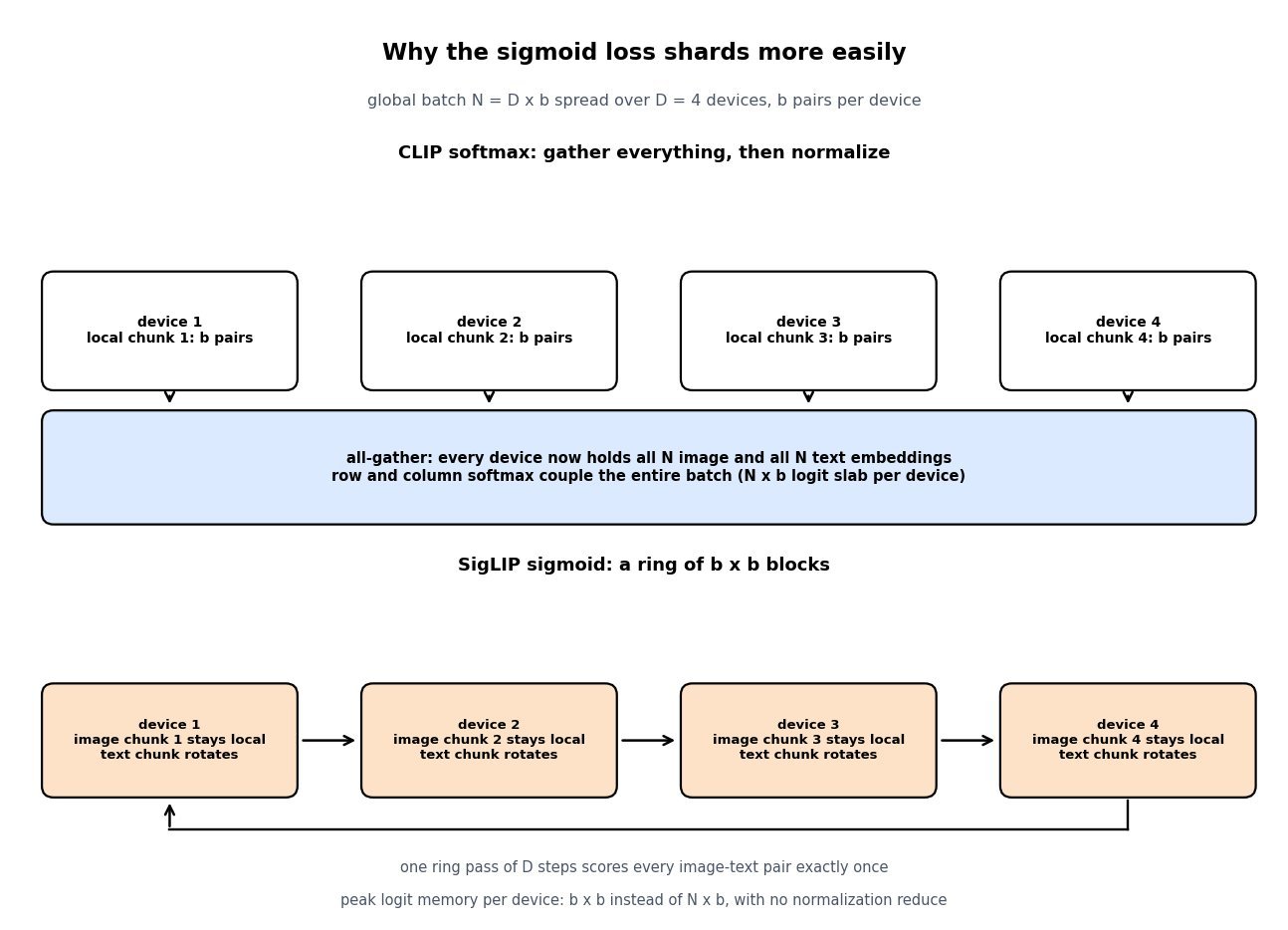
Top panel: four devices each holding a local chunk feed into an all-gather box where every device holds all N embeddings for a global softmax. Bottom panel: four devices keep their image chunk local while text chunks rotate around a ring, scoring one b by b block per step.

Figure 2: The softmax loss forces an all-gather and a global normalization, so each device carries an $N \times b$ logit slab. The sigmoid loss decomposes, so a ring of $D$ steps covers every pair while only $b \times b$ logits exist at once.

Property	SigLIP (sigmoid loss)	CLIP (softmax InfoNCE)
Objective	One binary logistic loss per image-text pair over the full grid	Two symmetric cross-entropies over row-wise and column-wise softmax
Batch coupling	None; the loss is a sum of independent terms	Global; every logit is normalized against the whole batch
Extra parameters	Learnable temperature plus a learnable bias, initialized to log 10 and -10	Learnable temperature only; a bias would cancel in the softmax
Distributed cost	Chunked ring; peak logit memory b x b per device, no normalization reduce	All-gather of all embeddings plus an N x b logit slab per device
Small batch (4k to 16k)	Clearly stronger zero-shot accuracy at equal examples seen	Degrades noticeably; the normalization has few negatives to work with
Very large batch	Feasible up to one million, but accuracy saturates near 32k	Comparable above roughly 32k, but memory-bound before that
Text context	64 tokens (16 in the original paper), 32k SentencePiece in the English releases	77 tokens, 49k byte-pair vocabulary
Typical role today	Default frozen vision tower for many VLMs, notably SoViT-400m/14	Legacy ecosystem: diffusion text conditioning, CLIPScore, many distilled models

August 17, 2026