Interview for Machine Learning

Category: Hard

DL0067 BERT VS GPT Pretraining
How does BERT’s pre-training objective differ from GPT’s?
Answer
BERT is trained primarily with masked language modeling: selected input tokens are corrupted, and a bidirectional encoder predicts the original tokens from visible context on both sides. GPT uses causal language modeling: a decoder predicts each next token using only earlier tokens, enforced by a triangular attention mask. MLM supplies loss only at selected positions and creates a corruption mismatch between pre-training and ordinary inputs, whereas causal modeling supplies a target at nearly every position and matches left-to-right generation. Original BERT also used next sentence prediction, while standard GPT pre-training relies on the autoregressive token objective rather than NSP.

Figure 1: BERT reconstructs selected corrupted tokens from two-sided context, while GPT predicts the next token at every step from a left-only prefix.
(1) Context Visibility: BERT’s visible tokens attend bidirectionally; GPT position $t$ cannot attend to positions later than $t$ .
(2) Prediction Targets: BERT reconstructs a selected masked subset, while GPT shifts the sequence and predicts the next token at each usable position.
(3) Downstream Bias: BERT naturally supports full-context understanding, whereas GPT’s objective directly trains open-ended autoregressive generation; either family can be adapted beyond that bias.
Mathematical Formulation:
$\mathcal{L}_{\mathrm{BERT}}=-\sum_{i\in\mathcal{M}}\log p(x_i\mid x_{\setminus\mathcal{M}})$
$\mathcal{L}_{\mathrm{GPT}}=-\sum_{t=1}^{T}\log p(x_t\mid x_{1:t-1})$
Where:
$\mathcal{L}_{\mathrm{BERT}}$ and $\mathcal{L}_{\mathrm{GPT}}$ are the masked and causal language-modeling losses.
$\mathcal{M}$ is BERT’s selected target set and $i\in\mathcal{M}$ indexes one target token $x_i$ .
$x_{\setminus\mathcal{M}}$ denotes BERT’s visible corrupted context outside the selected targets, and $p(x_i\mid x_{\setminus\mathcal{M}})$ is the reconstruction probability.
$t\in\{1,\ldots,T\}$ indexes a GPT target position, $T$ is sequence length, and $x_{1:t-1}$ is the preceding token prefix.
$p(x_t\mid x_{1:t-1})$ is the next-token probability and $\log$ converts each probability into a log-likelihood term.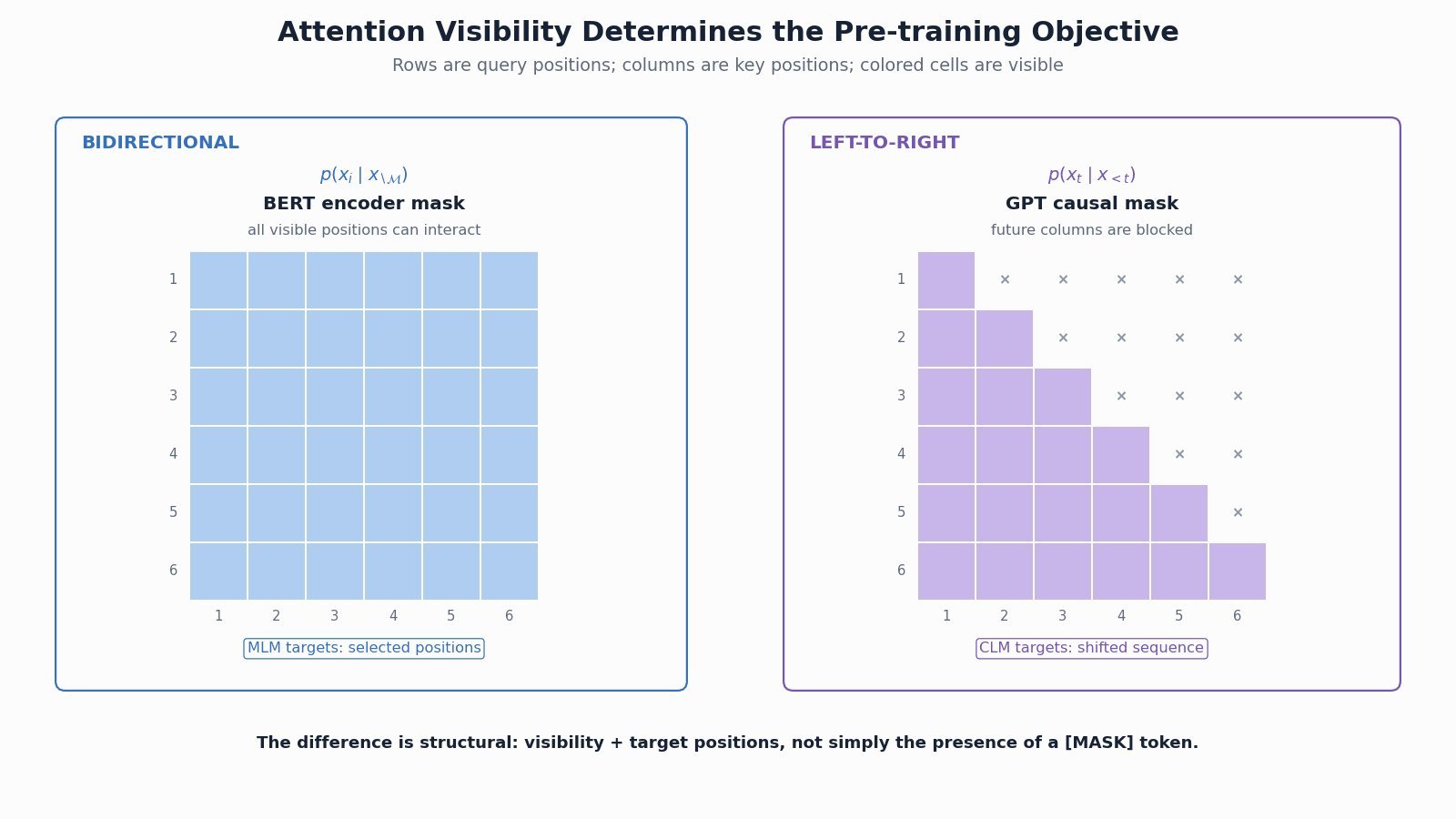

Figure 2: Attention visibility explains the objective difference: BERT uses a full visible-context matrix, while GPT uses a lower-triangular causal matrix.
Login to view more content
July 20, 2026
DL0056 FlashAttention
Explain FlashAttention. Why can it compute exact attention faster while using less memory?
Answer
FlashAttention is an exact, IO-aware implementation of scaled dot-product attention. Instead of materializing the full $N\times N$ score and probability matrices in high-bandwidth memory (HBM), it loads blocks of $Q$ , $K$ , and $V$ into fast on-chip SRAM, computes attention block by block, and maintains online softmax statistics. Tiling reduces expensive HBM reads and writes, while recomputation during the backward pass can be cheaper than storing large intermediates. The mathematical result matches standard attention up to normal floating-point differences; the speedup comes from changing the execution schedule, not from approximating attention.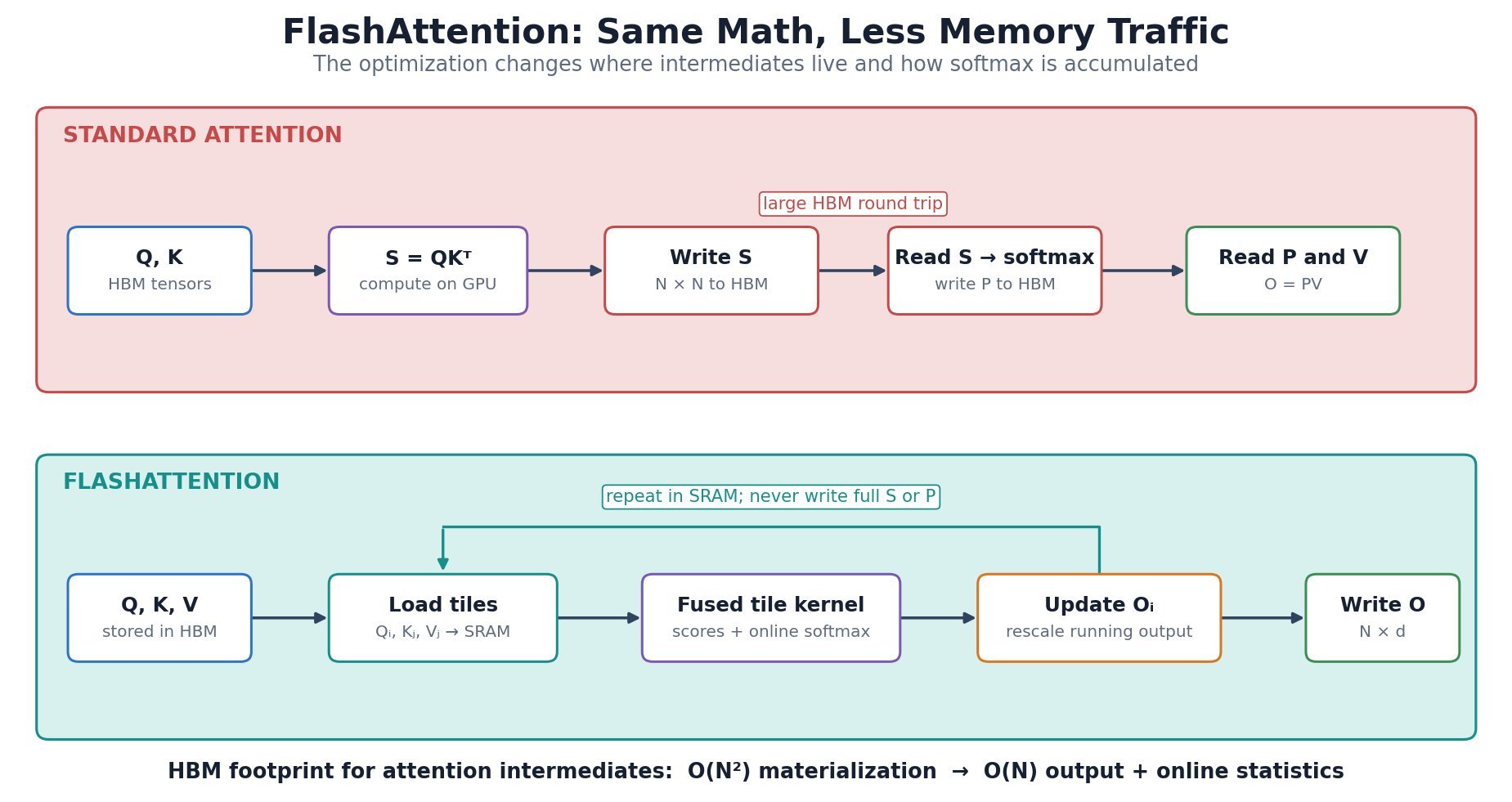

Figure 1: IO comparison showing why avoiding N×N intermediate writes makes FlashAttention faster and more memory efficient.
(1) IO Awareness: The kernel is organized around the GPU memory hierarchy so most score computation and softmax updates happen in SRAM.
(2) Online Softmax: A running row maximum and normalization sum allow each $K,V$ tile to update the output without retaining previous score blocks.
(3) Exact Result: All query-key interactions are evaluated; causal masking, dropout, and backward gradients are fused into specialized kernels rather than approximated.
Mathematical Formulation:
$m_i^{(t)}=\max\!\left(m_i^{(t-1)},\max_j S_{ij}^{(t)}\right)$
$\ell_i^{(t)}=e^{m_i^{(t-1)}-m_i^{(t)}}\ell_i^{(t-1)}+\sum_j e^{S_{ij}^{(t)}-m_i^{(t)}}$
Where:
$t$ indexes key/value tiles, $i$ indexes a query row, and $j$ indexes keys inside tile $t$ .
$S_{ij}^{(t)}=Q_iK_j^T/\sqrt d$ is the scaled score between query row $Q_i$ and key row $K_j$ , with head width $d$ .
$m_i^{(t)}$ is the running row maximum after tile $t$ , initialized with $m_i^{(0)}=-\infty$ .
$\ell_i^{(t)}$ is the running softmax denominator, initialized with $\ell_i^{(0)}=0$ ; the exponential factors rescale earlier partial sums when the maximum changes.

Figure 2: Blockwise FlashAttention loop with running maximum, normalization, output rescaling, and final HBM write.
Login to view more content
July 20, 2026
DL0039 Transformer Weight Tying
Explain weight sharing in Transformers.
Answer
Weight sharing in Transformers mainly refers to tying the input embedding matrix with the output projection matrix for softmax prediction, saving parameters, and improving consistency. In some models (like ALBERT), it also extends to sharing weights across Transformer layers for further parameter efficiency.
(1) Input–Output Embedding Tying:
The same embedding matrix is used for both input token embeddings and the output softmax projection.
Reduces parameters and enforces consistency between input and output spaces.
$\mbox{Softmax}(z_i) = \frac{e^{z_i}}{\sum_{j=1}^{K} e^{z_j}}$
Where:
$z_i = (E h)_i$ is the logit for token $i$ , computed using the embedding matrix $E \in \mathbb{R}^{K \times d}$ .
$h \in \mathbb{R}^{d}$ is the hidden representation from the Transformer.
$K$ is the vocabulary size.
Weights tying are shown in the figure below.
(2) Layer Weight Sharing (e.g., ALBERT [1]):
Instead of unique weights per layer, parameters are reused across all Transformer blocks.
Cuts model size dramatically while keeping depth.
References:
[1] Lan, Zhenzhong, et al. “Albert: A lite bert for self-supervised learning of language representations.” arXiv preprint arXiv:1909.11942 (2019).
Login to view more content
August 28, 2025
DL0033 Transformer Computation
In a Transformer architecture, which components are the primary contributors to computational cost, and why?
Answer
For short sequences, the feed-forward network (FFN) is often the dominant cost. For long sequences, the multi-head attention mechanism becomes the overwhelming bottleneck.
(1) Multi‑Head Attention (MHA):
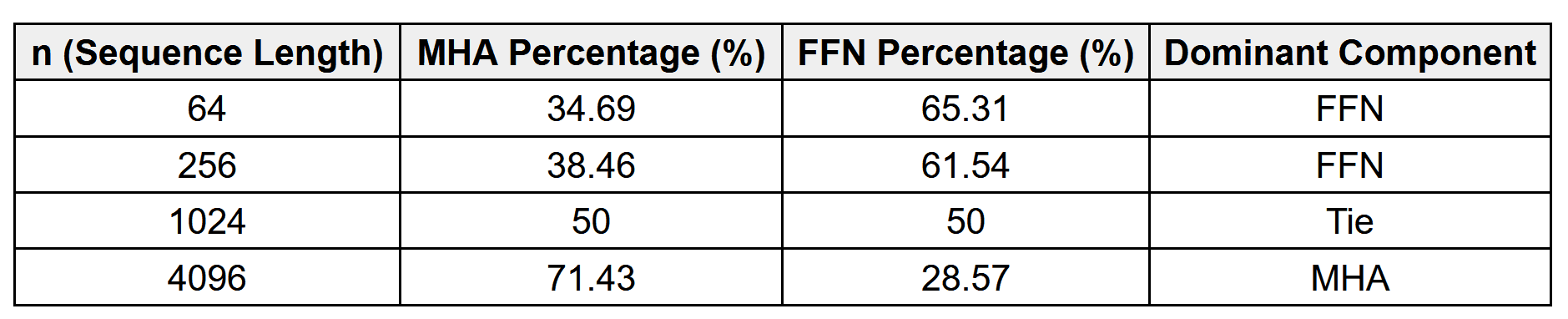
Short sequences (small $n$ ): Cost is relatively small; attention score matrix overhead is minimal. Q, K, and V projections together dominate the compute.
Long sequences (large $n$ ): Cost explodes quadratically with $n$ because every token attends to every other token. This becomes the main bottleneck. Cost: $\mathcal{O}(n^2 \cdot d)$
(2) Feed-Forward Network (FFN):
Two dense layers with an expansion factor of 4.
Cost: $\mathcal{O}(n \cdot d^2)$
Short sequences: FFN dominates cost since $n$ is small, but $d^2$ is large.
Long sequences: Cost grows linearly with $n$ , but MHSA cost overtakes it when $n$ is big.
The table below shows the FLOP breakdown comparing Multi‑Head Attention (MHA) and Feed‑Forward Network (FFN) at different sequence lengths for one of the transformer designs, where d=512.
Login to view more content
August 14, 2025