Tag: GenAI

DL0193 DINOv3 Frozen Backbone Zero-Shot Transfer

Why can DINOv3 perform zero-shot dense segmentation and classification using a completely frozen backbone without task-specific fine-tuning, and what properties of its self-supervised pretraining enable this transfer?

Answer

DINOv3 is pretrained with a purely discriminative self-distillation objective that supervises two granularities at once: an image-level DINO loss on the CLS token and a patch-level iBOT masked-latent loss on individual patch tokens. Because the target is another view’s latent assignment rather than a caption, patch tokens are never squeezed through a text bottleneck, so the $P \times d$ patch grid emerging from the last block is already a linearly separable semantic map rather than an intermediate code that only a trained decoder can read. The property that keeps this true at 7B parameters and 1.689B curated images is Gram anchoring: late in training DINOv3 adds a loss that matches the student’s patch-token Gram matrix to that of an earlier EMA teacher, pinning the patch-to-patch similarity structure while global features keep improving. Register tokens remove the high-norm artifact patches that otherwise pollute attention maps, and axial RoPE with frequency jittering makes the same weights usable at resolutions far above the training crop. The result is that read-out becomes non-parametric: k-NN on the CLS token classifies, and cosine similarity between patch embeddings segments, with no gradient ever entering the backbone. A single linear layer on the frozen features reaches roughly 88% ImageNet-1k top-1 and around 56 mIoU on ADE20k, which is why “frozen backbone plus tiny head” is a competitive deployment strategy rather than a baseline.

(1) Two Granularities Of Supervision: the DINO term shapes the CLS token for image-level tasks while the iBOT term shapes individual patch tokens, so dense and global capability are trained jointly instead of one being a by-product.
(2) No Text Bottleneck: contrastive image-text training pushes patch information toward one caption-level summary, whereas latent self-distillation leaves per-patch detail intact, which is exactly what dense matching consumes.
(3) Gram Anchoring Preserves Dense Structure: constraining the $P \times P$ similarity matrix, not the absolute features, lets representations keep drifting globally while patch-similarity geometry stays sharp.
(4) Artifact-Free High-Resolution Maps: register tokens absorb the global-information outliers that would otherwise appear as bright background patches, and jittered axial RoPE keeps features stable when inputs are upscaled.
(5) Read-Out Is Non-Parametric: cosine similarity to a handful of reference patches or a simple clustering of patch tokens yields masks with zero trained parameters, so “zero-shot” here is literal.
(6) Scale, Curation, Then Distillation: a 7B teacher on curated web data is distilled into ViT-S/B/L and ConvNeXt students that inherit the dense property, so the same recipe ships at deployable sizes.

Left-to-right diagram: an input image at any resolution passes through 16x16 patch embedding with four register tokens and jittered axial RoPE into a frozen ViT-7B/16 that receives no gradients, producing a CLS token and P patch tokens, which feed three read-out paths: k-NN or linear probe on the CLS token for ImageNet classification, patch-to-patch cosine similarity for zero-shot masks with no trained head, and a lightweight linear or DPT head for ADE20k segmentation and NYUv2 depth

Figure 1: One frozen backbone, three read-outs. The only task-specific parameters live to the right of the token boundary, and the middle path has none at all: it is pure cosine similarity between patch embeddings, which is only meaningful because Gram anchoring protected that similarity structure during pretraining.

The interesting failure this design fixes is temporal. Train DINO plus iBOT long enough at 7B scale and the two granularities diverge: image-level metrics such as ImageNet linear probing keep improving, while patch-level metrics (segmentation with a frozen linear head, video tracking, patch-similarity coherence) peak relatively early and then degrade. Patch tokens slowly become carriers of global, image-level evidence, so neighbouring patches on the same object stop being each other’s nearest neighbours and background patches start matching foreground ones. Monitoring only ImageNet accuracy hides this completely, which is why the effect went unaddressed for so long. Gram anchoring intervenes on the second-order statistic rather than the features: the student must reproduce the teacher’s patch-patch cosine matrix, so it is free to rotate, rescale, or refine the embedding space while the relational geometry that dense tasks read out is held in place. Meta reports the anchoring loss switched on in a late phase of training, using a Gram teacher whose features are computed at higher resolution and downsampled, which sharpens the target further.

Dual-axis schematic line chart over 1.2 million training iterations: the ImageNet-1k linear probe top-1 curve rises monotonically from about 76 to 88 percent, while the ADE20k frozen linear mIoU curve rises to about 56 by 0.22 million iterations, decays to about 48 by 1.0 million, then jumps back above 56 after a dash-dot vertical line marking where Gram anchoring is switched on

Figure 2: Schematic shape of the reported trend. Global and dense quality diverge under long self-supervised training, so a model that looks strictly better on classification can be strictly worse for zero-shot dense read-out. Gram anchoring recovers the dense curve without sacrificing the global one.

Mathematical Formulation:
$\mathcal{L} = \mathcal{L}_{\mathrm{DINO}} + \mathcal{L}_{\mathrm{iBOT}} + \lambda \mathcal{L}_{\mathrm{Gram}}$
$G_S = \hat{X}_S \hat{X}_S^{\top}$
$\mathcal{L}_{\mathrm{Gram}} = \| G_S - G_T \|_F^2$
$P = (H/16) \times (W/16)$
$s_{pq} = \hat{x}_p^{\top} \hat{r}_q$
$\hat{y}_p = \arg\max_q s_{pq}$

Where:

$\mathcal{L}_{\mathrm{DINO}}$ is the image-level cross-view self-distillation loss on the CLS token and $\mathcal{L}_{\mathrm{iBOT}}$ the patch-level masked-latent loss, with $\lambda$ weighting the anchoring term.
$\hat{X}_S \in \mathbb{R}^{P \times d}$ holds the student’s $L_2$ -normalized patch features and $\hat{X}_T$ the same for the Gram teacher, an earlier EMA checkpoint evaluated at higher resolution and downsampled.
$G_S, G_T \in \mathbb{R}^{P \times P}$ are the patch-patch cosine similarity matrices, so the loss constrains relations between patches and not the patch vectors themselves.
$P$ is the number of patch tokens for an $H \times W$ input at patch size 16, and $d$ the model width; the anchoring loss therefore costs $O(P^2 d)$ per view.
$\hat{x}_p$ is the normalized embedding of test patch $p$ and $\hat{r}_q$ a normalized reference embedding, taken from an annotated patch, a class prototype, or a cluster centroid.
$\hat{y}_p$ is the predicted label for patch $p$ ; the read-out has no learned weights, and the backbone is evaluated with $\lambda$ and all pretraining machinery discarded.

Two side-by-side grayscale heatmaps of cosine similarity to a single query patch marked by a red square inside a large elliptical object; the left map is sharp with high similarity confined to the object and near-zero elsewhere including on a nearby distractor object, while the right map is blurred and noisy with spurious high-similarity patches scattered across the background

Figure 3: What one row of $G$ looks like in image space. Zero-shot dense segmentation is nothing more than thresholding or arg-maxing maps like these, so map sharpness is the capability: the right-hand panel, typical of dense degradation, produces masks that bleed into the background even though the model’s classification accuracy is higher.

Two practical consequences follow. First, “zero-shot” in this setting means no text alignment: DINOv3 can tell you that patch $p$ belongs to the same thing as your reference patch, but it cannot be queried with the string “traffic cone” the way SigLIP or CLIP can, so open-vocabulary work still needs a language-aligned encoder or a small aligner trained on top. Second, freezing is what makes the model economical to operate: one forward pass produces features that many heads share, features can be cached, and there is no risk of catastrophic forgetting when a new task arrives.

Property	Frozen DINOv3	Frozen CLIP / SigLIP	Supervised fine-tuning
Pretraining signal	Self-distillation on images only, image-level plus patch-level	Image-text contrastive or sigmoid loss on alt-text pairs	Task labels, one dataset at a time
Patch-token quality	High and explicitly protected by Gram anchoring	Weaker: detail is compressed toward the caption-level summary	High for the trained task, unreliable off-task
Zero-shot dense masks	Yes, by cosine matching or clustering of patch tokens	Poor without a dense-adaptation stage	Not applicable, the head defines the label set
Text queries	None, references must be visual examples	Native open-vocabulary querying	Fixed closed vocabulary
Adaptation cost	Cache features once, train a linear or DPT head in minutes	Cheap for classification, expensive for dense tasks	Full backbone gradients per task, plus a new checkpoint
Dominant failure mode	Domains far from curated web imagery, and no semantics for text prompts	Blurred patch features and prompt sensitivity	Catastrophic forgetting and per-task serving cost

August 20, 2026

DL0186 Energy-Based Models and Contrastive Divergence

What is the Energy-Based Model (EBM) formulation, and how does Contrastive Divergence approximate the intractable partition function gradient without sampling full Markov chains?

Answer

An energy-based model refuses to parameterize a normalized density directly. It learns only a scalar energy function $E_{\theta}(x)$ , low for plausible configurations and high for implausible ones, and recovers a density by exponentiating and normalizing. The price of that freedom is the partition function $Z(\theta)$ , an integral over the whole input space that is intractable for anything beyond a toy problem. Differentiating the log-likelihood splits into a positive phase that lowers energy at observed data and a negative phase that raises energy wherever the model currently places mass, and the negative phase is an expectation under $p_{\theta}$ that normally needs MCMC samples at equilibrium. Contrastive divergence keeps the same two-phase update but initializes the chain at the training data rather than at noise, then runs only $k$ transition steps, in practice $k = 1$ . The estimate is biased because the $k$ -step distribution is not the equilibrium one, yet the bias shrinks near the optimum where the data distribution is already close to a fixed point of the sampler, and the variance is far lower than that of a long chain.

(1) Energy, Not Probability: the network outputs one unconstrained scalar per input, so any architecture works and no normalization layer or invertibility constraint is required.
(2) The Partition Function Is The Whole Problem: $Z(\theta)$ is a sum or integral over every possible configuration, so exact likelihood and exact sampling are both out of reach.
(3) Positive And Negative Phase: the exact gradient is a difference of two expectations of $\nabla_{\theta}E$ , one under the data and one under the model, which is why training is often described as pushing energy down at real points and up at fantasy points.
(4) Chain Started At The Data: CD replaces the equilibrium expectation with samples from a chain seeded at $x^{+}$ , which already sits in a high-probability region, so a very short run produces a usable contrast.
(5) Truncation Trades Bias For Cost: per-update cost drops from a full mixing time to $k$ transitions, at the cost of a systematically biased gradient that ignores model mass far from the data.
(6) CD Is An Update Rule, Not A True Gradient: the CD-1 update is not the exact gradient of any objective function, so convergence guarantees are weak and divergence is possible in principle.

Flow diagram with a top lane showing a data batch feeding the positive phase that lowers energy at the data point, and a bottom lane where the same data point initializes a Markov chain of k short steps producing the negative sample, with both phases feeding a single parameter update box

Figure 1: The two-phase update. Exact maximum likelihood would draw the negative sample from the model at equilibrium, costing a full chain run per parameter update. CD keeps the identical update form but seeds the chain at the data and stops after $k$ steps, which turns an expensive unbiased gradient into a cheap biased one.

Mathematical Formulation:
$p_{\theta}(x) = \frac{e^{-E_{\theta}(x)}}{Z(\theta)}$
$Z(\theta) = \int e^{-E_{\theta}(x)}\,dx$
$\log p_{\theta}(x) = -E_{\theta}(x) - \log Z(\theta)$
$\nabla_{\theta}\log Z(\theta) = -\mathbb{E}_{p_{\theta}}[\nabla_{\theta}E_{\theta}]$
$\nabla_{\theta}\mathcal{L} = \mathbb{E}_{p_{\mathrm{data}}}[\nabla_{\theta}E] - \mathbb{E}_{p_{\theta}}[\nabla_{\theta}E]$

Where:

$p_{\theta}(x)$ is the model density and $E_{\theta}(x) \in \mathbb{R}$ the learned energy, with lower energy meaning higher probability.
$Z(\theta)$ is the partition function, an integral over the full input space (a sum for discrete $x$ ) that depends on $\theta$ and therefore cannot be ignored during training.
$x$ is a configuration and $\theta$ the parameters of the energy network.
$\mathcal{L} = -\mathbb{E}_{p_{\mathrm{data}}}[\log p_{\theta}]$ is the average negative log-likelihood, so the first expectation is the positive phase and the second is the negative phase.
The identity $\nabla_{\theta}\log Z = -\mathbb{E}_{p_{\theta}}[\nabla_{\theta}E]$ is what converts an intractable normalizer into an expectation, which is exactly why sampling becomes the bottleneck.

The Contrastive Divergence Approximation:
$p_k = p_0 T_{\theta}^{k}$
$\nabla_{\theta}\mathcal{L}_{\mathrm{CD}} = \mathbb{E}_{p_0}[\nabla_{\theta}E] - \mathbb{E}_{p_k}[\nabla_{\theta}E]$
$\mathcal{L}_{\mathrm{CD}} \approx D_{KL}(p_0 \| p_{\theta}) - D_{KL}(p_k \| p_{\theta})$

Where:

$p_0 = p_{\mathrm{data}}$ is the empirical distribution used as the chain initialization, and $p_k$ is the distribution after $k$ applications of the transition operator.
$T_{\theta}$ is any transition operator leaving $p_{\theta}$ invariant, typically block Gibbs for an RBM or Langevin dynamics for a continuous EBM.
$k$ is the truncation depth, with $k = 1$ the standard choice and larger $k$ reducing bias at linear cost.
As $k \to \infty$ we recover $p_k = p_{\theta}$ and the update becomes the exact likelihood gradient, so CD is a controllable interpolation between a free estimate and an unbiased one.
The two-KL form is the original motivation rather than an exact objective; a small ignored term involving $\partial p_k / \partial \theta$ is what makes CD not the gradient of any function.

The restricted Boltzmann machine is the case where every piece is closed-form, which is why CD was invented there. Because there are no visible-visible or hidden-hidden couplings, the conditionals factorize completely and one Gibbs sweep is a single pass of matrix multiplies plus sigmoids, following the chain v → h → v’ → h’. CD-1 then reduces to the difference between a data correlation and a reconstruction correlation, computable with two forward passes and no backpropagation through a sampler.

Binary RBM Case:
$E_{\theta}(v,h) = -v^{\top}Wh - b^{\top}v - c^{\top}h$
$p(h_j = 1 \mid v) = \sigma(c_j + W_{:j}^{\top}v)$
$\Delta W = \eta\,(v_0 h_0^{\top} - v_1 h_1^{\top})$

Here $v_0$ is the data vector, $h_0 \sim p(h \mid v_0)$ , and $(v_1, h_1)$ come from one further Gibbs sweep. The positive term raises the weight between co-active data units and the negative term subtracts the same statistic measured on the model’s one-step reconstruction, so learning stops precisely when the reconstruction statistics match the data statistics.

One-dimensional energy landscape curve with a deep data basin on the left and a spurious model basin on the right separated by a barrier, showing the data point where the positive phase lowers energy, the k-step chain sample nearby where the negative phase raises energy, and a distant full-chain sample in the spurious basin that a short chain never reaches

Figure 2: The structural blind spot. A $k$ -step chain started at $x^{+}$ stays inside the data basin, so the negative phase only ever penalizes points the model already ranks near the data. A spurious mode behind an energy barrier keeps its low energy indefinitely because CD never samples there, and this is why CD-trained models can assign high likelihood to garbage.

The practical consequences follow directly from that picture. Slow mixing is not a nuisance but the defining constraint, since the time to cross a barrier grows exponentially in its height, so raising $k$ from 1 to 20 buys much less than the cost suggests. Persistent CD attacks the same problem differently by keeping a set of chains alive across parameter updates instead of restarting them at data, which lets the fantasy particles drift into spurious regions given enough updates, at the cost of instability when the learning rate is large relative to the mixing rate. Modern continuous EBMs use short-run Langevin dynamics with a replay buffer plus gradient clipping and energy regularization, and increasingly avoid MCMC entirely through score matching or its denoising variant, which never touches $Z(\theta)$ because the score $\nabla_x \log p_{\theta}(x) = -\nabla_x E_{\theta}(x)$ is independent of the normalizer.

Property	CD-k	Persistent CD	Score matching
Negative sample source	k transitions from the current data batch	Persistent fantasy particles carried across updates	None; no sampling during training
Cost per update	k sweeps, usually one	One sweep, plus buffer memory	One or two extra backward passes for derivatives
Main bias or error	Truncation bias; distant spurious modes never penalized	Chains lag a moving target, so samples are stale	Consistent but blind to relative mass between separated modes
Stability	Very stable, low variance, forgiving of large learning rates	Needs a small learning rate so chains can keep up	Stable, but plain score matching struggles in high dimension without noise
Best fit	RBMs and discrete models with exact block Gibbs	Longer training runs where density quality matters more than speed	Continuous high-dimensional data, the route taken by diffusion models

August 20, 2026

DL0185 CycleGAN Cycle Consistency Loss

How does CycleGAN use Cycle Consistency Loss to train unpaired image-to-image translation, and what are its limitations regarding mode collapse and semantic preservation?

Answer

CycleGAN trains two generators at once, $G: X \to Y$ and $F: Y \to X$ , each with its own PatchGAN discriminator, using only samples from the two marginals $p_X$ and $p_Y$ and never a matched pair. The adversarial terms alone are hopelessly under-constrained, because any mapping whose pushforward equals $p_Y$ is optimal, including one that ignores the input entirely. The cycle consistency loss adds an $\ell_1$ reconstruction penalty in both directions, $F(G(x)) \approx x$ and $G(F(y)) \approx y$ , which forces the two generators to be approximate inverses and therefore rules out constant outputs and arbitrary re-pairing. The critical limitation is that this constraint is invariant to any label-permuting bijection: it enforces invertibility, not meaning, so a translation that swaps content while remaining perfectly reversible pays zero cycle loss. In practice this shows up as residual per-mode collapse (one stripe pattern for every horse), self-adversarial steganography (imperceptible high-frequency codes that let $F$ cheat), and semantic hallucination such as painting zebra texture onto a rider or inventing a lesion in a medical scan.

(1) Two Coupled Mappings, Four Networks: $G$ , $F$ , $D_Y$ , and $D_X$ train jointly, with the adversarial terms fixing the target marginal and nothing else.
(2) Cycle Loss As A Soft Bijection: a bidirectional $\ell_1$ reconstruction penalty weighted by $\lambda = 10$ ties the two generators into an approximate inverse pair.
(3) What It Genuinely Prevents: total collapse is impossible, since a generator that emits one fixed image destroys all input information and $F$ cannot reconstruct $x$ from it.
(4) What It Does Not Constrain: composing $G$ with any measure-preserving permutation of the target domain leaves both losses unchanged, so semantics is unconstrained and only the convolutional inductive bias keeps translations sane.
(5) Self-Adversarial Steganography: the pair can hide a low-amplitude code in the output so reconstruction is near-perfect while the visible translation is wrong, making cycle loss a weak proxy for content preservation.
(6) Deterministic One-To-One Bias: cycle consistency actively penalizes information loss, so many-to-one tasks and geometric or shape changes fail while texture and color remapping succeeds.

Diagram of the CycleGAN objective with a top row showing a real horse photo passing through generator G to a fake zebra and then through generator F back to a reconstruction, a bottom row showing the reverse cycle from a real zebra through F and G, dashed routed paths marking the two L1 cycle losses, and two discriminator boxes in the middle band receiving the fake samples

Figure 1: The full objective in one view. The adversarial terms only ask whether $G(x)$ looks like some member of domain $Y$ , and the cycle terms only ask whether the round trip returns to the start, so no term in the loss ever compares a translated horse against the true zebra version of that same horse.

The published recipe matters because most of the stability comes from implementation choices rather than from the loss on paper. The generators are ResNet encoders with 9 residual blocks at $256 \times 256$ resolution, the discriminators are $70 \times 70$ PatchGAN critics that score local patches instead of the whole image, and the adversarial term uses the least-squares (LSGAN) form rather than the log-likelihood form to avoid vanishing gradients. Discriminators are updated against a buffer of 50 previously generated images, which damps oscillation, and training uses Adam at $2 \times 10^{-4}$ with batch size 1 and a linear learning-rate decay after the first 100 epochs. For photo and painting transfer an extra identity loss weighted at $0.5 \lambda$ penalizes $\|G(y) - y\|_1$ , which is a purely empirical patch that stops the generators from inverting the color palette.

Mathematical Formulation:
$\mathcal{L}_{\mathrm{GAN}}(G, D_Y) = \mathbb{E}_y[(D_Y(y) - 1)^2]$
$+ \mathbb{E}_x[D_Y(G(x))^2]$
$\mathcal{L}_{\mathrm{cyc}} = \mathbb{E}_x \| F(G(x)) - x \|_1$
$+ \mathbb{E}_y \| G(F(y)) - y \|_1$
$\mathcal{L} = \mathcal{L}_{\mathrm{GAN}}(G, D_Y) + \mathcal{L}_{\mathrm{GAN}}(F, D_X)$
$+ \lambda \mathcal{L}_{\mathrm{cyc}}$

Where:

$\mathcal{L}_{\mathrm{GAN}}(G, D_Y)$ is the least-squares adversarial term that $D_Y$ minimizes; the generator instead minimizes $\mathbb{E}_x[(D_Y(G(x)) - 1)^2]$ , which is the non-saturating counterpart.
$x \sim p_X$ and $y \sim p_Y$ are independent draws from the two marginals; there is no joint distribution over pairs anywhere in the objective.
$G$ and $F$ are the two generators, $D_X$ and $D_Y$ the two patch discriminators, all four trained simultaneously.
$\mathcal{L}_{\mathrm{cyc}}$ sums the forward and backward reconstruction errors in $\ell_1$ , chosen over $\ell_2$ because it blurs less.
$\lambda$ is the cycle weight, set to 10 in the paper; raising it sharpens reconstruction and suppresses collapse, but it also makes the generator conservative and can push it toward hidden encodings.

Why The Constraint Is Semantically Blind:
$G' = T \circ G$
$F' = F \circ T^{-1}$
$T_{\#} p_Y = p_Y$
$\mathcal{L}(G', F') = \mathcal{L}(G, F)$

Take any invertible map $T$ on the target domain whose pushforward leaves $p_Y$ unchanged, for example a permutation that sends every image of a single zebra to an image of two zebras and vice versa. Then $G' = T \circ G$ produces samples with exactly the same distribution, so both discriminators are equally fooled, and $F' = F \circ T^{-1}$ still reconstructs the input exactly, so the cycle loss is unchanged. The two solutions are therefore indistinguishable global optima, and the one you actually get is decided by the generator’s limited receptive field, its residual skip structure, and the fact that near-identity mappings are easy to learn. That is a statement about architecture, not about the loss, which is why CycleGAN is reliable for texture and color transfer and unreliable the moment a task requires moving or removing structure.

Two side-by-side panels each showing three boxes of horse-photo content classes on the left and three boxes of zebra-photo content classes on the right; the left panel connects them with parallel content-preserving arrows while the right panel connects them with crossing permuted arrows, and both panels are annotated with identical zero cycle loss and matched marginals

Figure 2: Two mappings between the same two sets. Both are exact bijections and both match the target marginal, so adversarial loss and cycle loss are numerically identical, yet only the left one preserves content. Nothing in the CycleGAN objective distinguishes them, which is the formal root of label flipping and hallucination.

Property	CycleGAN (cycle loss)	CUT (patchwise contrastive)	CycleGAN-Turbo (one-step diffusion)
Content constraint	Round-trip $\ell_1$ reconstruction in both directions	PatchNCE: a patch must match its own location across the translation	Cycle plus perceptual identity on top of a pretrained text-to-image prior
Networks trained	Two generators plus two discriminators	One generator, one discriminator, one small projection head	LoRA adapters on a frozen one-step diffusion backbone
Training cost	Highest of the three: four forward passes per step	Roughly half the memory, single-direction training	Low trainable parameter count, but a large frozen backbone in memory
Output diversity	Deterministic, one output per input by construction	Deterministic, but no invertibility pressure to preserve everything	Deterministic at one step, though the prior supplies plausible detail
Characteristic failure	Hidden encodings, label flipping, refusal to change shape	Weaker global structure retention when the patch head is mistuned	Inherits the prior’s biases and hallucinates plausible but absent detail

August 20, 2026

DL0177 Discrete vs Continuous Visual Tokens

What is the difference between discrete visual tokenization (e.g., VQ-VAE, VQ-GAN) and continuous vision embeddings (e.g., ViT patch outputs), and when is each preferred for generation versus understanding tasks?

Answer

Both paths begin identically, with a convolutional or ViT encoder turning the image into a grid of $d$ -dimensional vectors. The only structural difference is whether a quantizer follows. A discrete tokenizer (VQ-VAE, VQ-GAN) snaps each vector to its nearest entry in a learned codebook of $K$ vectors and keeps only the integer index, so an image becomes a string of ids over a finite vocabulary that a jointly trained decoder can invert back to pixels. A continuous representation (ViT patch outputs, CLIP or SigLIP features, KL-VAE latents) keeps the float vector, which preserves far more information but has no finite support, so no softmax and no cross-entropy can be defined over it. That single difference decides the downstream interface: discrete ids plug into next-token or masked-token prediction with exactly the machinery used for text, while continuous features must be projected into an LLM or denoised by a diffusion model. As a default, understanding prefers continuous features because quantization discards the high-frequency detail that OCR and fine-grained VQA depend on, while generation historically preferred discrete tokens because a categorical likelihood is easy to train and easy to sample.

(1) Only The Quantizer Differs: the encoder, the patch grid, and the spatial downsampling factor can be identical; adding a nearest-code lookup converts a float grid into an id grid.
(2) Information Budget: a discrete token carries $\log_2 K$ bits (10 to 18 in practice), while a continuous patch vector carries roughly $d \times 16$ bits of activation, three orders of magnitude more.
(3) Gradient Path: $\arg\min$ is non-differentiable, so VQ needs a straight-through estimator plus codebook and commitment losses, whereas continuous encoders train by plain backpropagation.
(4) Reconstruction Cost: heavy compression makes plain L2 reconstruction blurry, which is why VQ-GAN adds perceptual and patch-GAN losses to keep 16x-downsampled decodes sharp.
(5) Downstream Interface: discrete gives one softmax vocabulary shared with text; continuous gives features for a projector, cross-attention, or a latent diffusion denoiser.
(6) Task Split: continuous features dominate VLM understanding benchmarks; discrete tokens dominate when the goal is a single unified next-token model that also emits pixels.

Two horizontal pipelines: the upper understanding path runs input image to ViT patch encoder to 256 continuous vectors in R^1024 to a linear projector to an LLM emitting text, with no quantizer and no pixel decoder; the lower generation path runs input image to a CNN or ViT encoder to a quantizer that picks the nearest of K codes, to a 16 by 16 grid of integer ids, to a transformer with a softmax over K, to a decoder producing pixels

Figure 1: The same encoder, two endings. Deleting the quantizer leaves continuous features that a projector feeds to an LLM; inserting it buys a finite vocabulary and a pixel decoder at the price of $\log_2 K$ bits per token. Note that the understanding path has no decoder at all, which is why an understanding-only encoder is never required to be invertible.

The practical difficulty of discrete tokenization is that the codebook must be learned through a non-differentiable lookup. The straight-through estimator simply copies the decoder gradient past the quantizer, which is a biased estimate that works only if the encoder output stays close to its assigned code, hence the commitment loss. The characteristic failure is codebook collapse: a few entries win most assignments, the rest receive no gradient and die, and effective vocabulary size stops tracking nominal $K$ . Standard mitigations are EMA codebook updates, low-dimensional $\ell_2$ -normalized codes, dead-code re-initialization, and an entropy bonus on the assignment distribution. Continuous encoders have none of this machinery, but they also cannot be sampled from, since there is no distribution over $\mathbb{R}^{d}$ that a softmax can express, which is precisely why continuous-latent generation requires a diffusion or flow model rather than a token classifier.

Mathematical Formulation:
$z = E(x)$
$k = \arg\min_{j} \lVert z - e_j \rVert_2$
$z_q = e_k$
$\hat{x} = D(z_q)$
$\mathcal{L}_{\mathrm{com}} = \beta \lVert z - \mathrm{sg}(e_k) \rVert_2^2$

Where:

$x$ is the input image, $E$ the encoder, and $z \in \mathbb{R}^{d}$ one continuous patch vector from the encoder grid; keeping $z$ and stopping here is the continuous path.
$e_j$ for $j \in \{1,\ldots,K\}$ are the learned codebook vectors, $k$ is the selected index (the actual token), and $K$ is the vocabulary size.
$z_q$ is the quantized vector fed to the decoder $D$ , and the residual $z - z_q$ is information the model can never recover.
$\mathrm{sg}(\cdot)$ is the stop-gradient operator and $\beta$ (typically $0.25$ ) weights the commitment loss that pulls encoder outputs toward their assigned codes.
The full VQ-GAN objective adds a reconstruction term, an LPIPS perceptual term, and a patch-discriminator term to $\mathcal{L}_{\mathrm{com}}$ ; only the reconstruction term survives in a plain VQ-VAE.

Bit Budget For One 256×256 Image:
$B_{\mathrm{disc}} = 256 \times 14 = 3584$
$B_{\mathrm{cont}} = 256 \times 1024 \times 16$
$B_{\mathrm{cont}} = 4194304$
$B_{\mathrm{cont}} / B_{\mathrm{disc}} \approx 1170$

All four numbers are in bits. A 16x-downsampling tokenizer with $K = 16384$ compresses the image to 256 ids of 14 bits each, about 448 bytes, while a ViT-L/14 tower keeps 256 patch vectors of 1024 bf16 activations, about 512 KiB. That ratio is the whole argument: it is why a discrete sequence is short enough to model autoregressively alongside text, and equally why an OCR-heavy or chart-reading task should not be routed through it.

Left panel shows a two-dimensional scatter of continuous encoder outputs partitioned into nine square cells by dashed boundaries, with a black X codebook entry at each cell center and one highlighted red point joined by an arrow to its nearest code, labelled quantization error. Right panel plots reconstruction FID against bits per token from 10 to 18, with a plain VQ curve that stalls near 5 and rises after 14 bits, a lookup-free or FSQ curve that keeps falling toward 1.2, and a dashed horizontal line marking the continuous KL-VAE floor near 0.74

Figure 2: Left, quantization is a Voronoi partition of the latent space: the id names the cell, and the offset inside the cell is thrown away. Right, approximate published reconstruction results show that a plain VQ codebook stops improving past about $2^{14}$ entries because of codebook collapse, whereas lookup-free and FSQ-style quantizers keep scaling toward the continuous-latent floor.

Property	Discrete (VQ-VAE / VQ-GAN)	Continuous (ViT / KL-VAE)
What a token is	An integer index into a learned codebook of K vectors	An unconstrained d-dimensional float vector
Information per token	log2 K bits, typically 10 to 18	About d x 16 bits, typically 4k to 16k
Gradient path	Non-differentiable argmin, needs a straight-through estimator plus commitment loss	Plain end-to-end backpropagation
Known instability	Codebook collapse and dead codes, with usage often below 10 percent at large K	Latent scale drift without a KL term or normalization
Generation interface	Cross-entropy over K, autoregressive or masked sampling, one vocabulary shared with text	Latent diffusion or flow matching, or a small per-token diffusion head
Understanding quality	Weaker OCR, charts, and fine-grained recognition after the bottleneck	Default choice: CLIP or SigLIP features feed the projector in most VLMs
Pixel decoder	Required, trained jointly with the codebook	Only if the task emits pixels; understanding-only towers have none

August 19, 2026

DL0167 Video Generation Physical Consistency Evaluation

How do you evaluate physical consistency (gravity, collision, object permanence, and temporal coherence) in video and world generation models beyond standard distributional metrics like FID and FVD?

Answer

FID and FVD compare summary statistics of clip embeddings from appearance-biased backbones (InceptionV3, I3D), so they answer whether a set of generated videos resembles a reference set, never whether one clip obeys physics. They are dominated by per-frame content rather than motion, they are nearly insensitive to short-range frame reordering, and they can improve while dynamics get worse. Physical consistency therefore needs per-clip, falsifiable probes. The three that work in practice are: condition the model on the opening frames of a real recorded event and score the predicted continuation against the actual future; ask a calibrated judge (human, or a VLM validated against human labels) for a binary physical-commonsense verdict on each clip; and extract a symbolic readout (track → lift to 3D → fit dynamics) so gravity, momentum, permanence, and flow coherence become numbers with known correct values. For a world model you add a fourth layer, closed-loop rollout, because the only decision-relevant question is whether a policy trained or planned inside the model still succeeds in the real environment.

(1) Distributional vs Per-Clip: FVD is a set-level Frechet distance and cannot label a single video as physically wrong, so it belongs in a regression suite, not in a physics report.
(2) Real-Continuation Probes: give the model the first frames of a genuine recorded event and compare the continuation to ground truth with spatial IoU of the motion mask and masked pixel MSE.
(3) Calibrated Judges: report physical commonsense (PC) and semantic adherence (SA) separately plus their joint pass rate, and publish the judge’s agreement with humans before trusting it.
(4) Symbolic Readout: tracking plus depth lifting turns physics into scalars: fitted gravity residual, momentum error at collisions, occlusion recovery rate, and optical-flow warp error.
(5) Object Permanence Is A Timeline Test: it is only measurable across an occlusion window, so probes must be authored with an occluder and scored on identity, count, and attribute preservation after reappearance.
(6) Closed-Loop For World Models: action-conditioned rollouts are scored by drift over horizon and downstream task success, which is the metric that actually correlates with usefulness.

Diagram of a four-tier evaluation stack: a generated clip with its conditioning fans out to tier one distributional FID and FVD over I3D features, tier two real-continuation probe comparing to a recorded future, tier three calibrated human or VLM judge giving a binary per-clip verdict, and tier four symbolic readout that tracks objects and fits dynamics; each tier emits its own metrics and tiers two to four feed a per-clip physics scorecard while tier one connects with a dashed arrow

Figure 1: The evaluation stack. Only tiers 2 to 4 return a verdict for an individual clip; tier 1 is a distribution-level sanity check whose score can fall (improve) while gravity and collision behaviour degrade, which is exactly why it is drawn with a dashed contribution.

Each of the four physical axes needs a different probe design. Gravity is measured by tracking a free-falling centroid, fitting a quadratic to its height, and comparing the implied acceleration to the reference: generated video overwhelmingly fails toward floaty, slow-motion dynamics with a fitted value well below the true one. Collision is measured at the impact frame, where you check momentum and energy: a coefficient of restitution above 1, interpenetration, or objects passing through each other are hard violations that no appearance metric sees. Object permanence requires a prompt authored with an occluder, then a check that the object reappears with the same identity, count, and colour; the natural scores are the recovery rate and identity-switch count borrowed from multi-object tracking. Temporal coherence is the cheapest to automate: warp consecutive frames with optical flow, mask out occlusions and disocclusions, and average the residual, which catches flicker, texture swimming, and morphing that a per-frame FID is blind to. Crucially, all four scores are reported as per-clip pass rates over a curated probe set, not as an average of a continuous score, because averaging hides the fact that most failures are categorical.

Mathematical Formulation:
$d_F^2 = \| \mu_r - \mu_g \|_2^2 + T_{\Sigma}$
$T_{\Sigma} = \mathrm{Tr}(\Sigma_r + \Sigma_g - 2 (\Sigma_r \Sigma_g)^{1/2})$
$y(t) = y_0 + v_0 t + \frac{1}{2} \hat{g} t^2$
$e_g = | \hat{g} - g | / g$
$e_p = \| p^{+} - p^{-} \| / \| p^{-} \|$
$R_p = N_{\mathrm{rec}} / N_{\mathrm{occ}}$
$\tilde{I}_t = \mathcal{W}(I_t, f_{t \to t+1})$
$\epsilon_t = \| m_t \odot (I_{t+1} - \tilde{I}_t) \|_1$
$E_w = \frac{1}{T-1} \sum_{t=1}^{T-1} \epsilon_t$
$J = \frac{1}{N} \sum_{i=1}^{N} c_i^{\mathrm{pc}} c_i^{\mathrm{sa}}$

Where:

$d_F^2$ is the FVD value, with $\mu_r, \Sigma_r$ and $\mu_g, \Sigma_g$ the mean and covariance of real and generated clip features from a fixed video backbone; it is defined only over sets, which is the root of its uselessness for per-clip physics.
$y(t)$ is the tracked height of an object at time $t$ , $y_0$ and $v_0$ the fitted initial height and velocity, and $\hat{g}$ the least-squares acceleration recovered from the generated clip; $e_g$ is its relative error against the reference $g$ .
$p^{-}$ and $p^{+}$ are total momentum immediately before and after a contact frame, so $e_p$ is the relative momentum violation; the same construction on kinetic energy exposes a restitution above 1.
$N_{\mathrm{occ}}$ is the number of authored occlusion events and $N_{\mathrm{rec}}$ the number where the object reappears with correct identity, count, and attributes, giving the permanence recovery rate $R_p$ .
$\mathcal{W}$ is backward warping by the estimated flow $f_{t \to t+1}$ , $m_t$ the binary validity mask that removes occluded and out-of-frame pixels, $\odot$ elementwise product, and $E_w$ the averaged warp error over the $T$ frames.
$c_i^{\mathrm{pc}}, c_i^{\mathrm{sa}} \in \{0,1\}$ are the physical-commonsense and semantic-adherence verdicts on clip $i$ , so $J$ is the joint pass rate: a clip counts only if it is both on-prompt and physically plausible.

Two-panel chart. Left panel plots tracked height versus time for a reference bouncing ball following ballistic arcs with decaying apex heights and a generated clip that falls more slowly, dips below the floor line, and rebounds to an apex higher than its release height. Right panel plots speed magnitude versus time, showing the reference speed dropping from about 9.9 to 7.4 metres per second at impact while the generated clip's speed increases from about 6.6 to 7.6 metres per second at impact

Figure 2: The symbolic readout on one probe clip. The fitted acceleration is 4.2 instead of 9.8, the object interpenetrates the floor, and the post-impact speed exceeds the pre-impact speed (restitution above 1, so energy is created). Every one of these is a numeric, falsifiable failure; all of them are invisible to a distributional metric computed on the same clip.

Metric family	Granularity	What it catches	What it misses
FID / FVD	Set level, needs hundreds of clips	Gross artefacts, blur, mode collapse, distribution shift	All per-clip physics; content bias makes it track texture more than motion
Real-continuation probe	Per clip, against recorded ground truth	Wrong outcome of a near-deterministic event (where a ball lands, whether paint mixes)	Legitimate stochastic futures are penalised unless you score a sampled set
Calibrated human or VLM judge	Per clip, binary PC and SA	Open-ended violations on arbitrary prompts, including material and state-change errors	Sub-second and geometric violations; judge agreement with humans is far from perfect
Symbolic trajectory readout	Per clip, per object, per frame	Gravity residual, momentum and energy errors, interpenetration, identity switches, warp error	Anything the tracker or depth model cannot follow: fluids, smoke, cloth, heavy occlusion
Closed-loop rollout	Per episode, action-conditioned	Compounding drift and any error that actually changes a policy’s decision	Expensive, needs an action-conditioned model plus a real or simulated environment

August 19, 2026

DL0166 3D Gaussian and NeRF Neural Simulator

How do 3D Gaussians and Neural Radiance Fields serve as dense physical representations inside differentiable neural simulators?

Answer

A differentiable neural simulator needs one scene description that works twice: as geometry the solver can push around, and as an image the photometric loss can compare against real video. NeRF supplies the second half well, storing the scene as an implicit field that maps a position and view direction to density and radiance, rendered by differentiable volume quadrature along rays. What it lacks is handles, because an MLP field has no particle to give mass, no covariance to advect, and no obvious place to attach a constitutive model. 3D Gaussian Splatting removes that obstacle by storing the scene as an explicit set of anisotropic Gaussians with mean, covariance, opacity, and spherical-harmonic color, so every primitive doubles as a material point in a Lagrangian solver. The simulator advances those points with differentiable physics, usually MLS-MPM, the rasterizer splats them back to pixels, and gradients from the rendering loss flow through both the rollout and the renderer into material parameters such as Young’s modulus, Poisson ratio, yield stress, and friction. The loop is therefore video → physical parameters → rollout of unseen dynamics, with pixels as the only supervision.

(1) Dense Means Physics Everywhere: unlike a mesh, both representations describe the interior volume, so mass, velocity, and stress are defined at every sampled point rather than only on a surface shell.
(2) Gaussians Are Already Particles: a splat’s mean is a particle position and its covariance is a local volume element, which is exactly the state an MPM particle carries, so the reconstruction and the simulation share one data structure.
(3) NeRF Needs A Bridge: a continuous field has to be voxelized or resampled onto particles each step, the Eulerian-Lagrangian conversion that PAC-NeRF introduced, which costs an extra transfer and an extra source of gradient noise.
(4) Covariance Follows The Deformation Gradient: kinematics are preserved by advecting the mean through the flow map and conjugating the covariance with $F$ , otherwise stretched material still renders as undeformed blobs.
(5) The Loss Is Purely Photometric: no ground-truth stiffness is available, so system identification is driven by rendered-versus-observed pixel error over a multi-frame rollout.
(6) The Cost Lives In The Backward Pass: memory grows as $O(TN)$ in substeps and particles, and gradients through contact and friction are non-smooth, so checkpointing and softened contact models are mandatory.

Left-to-right pipeline: multi-view video with camera poses feeds a dense reconstruction stage producing 3D Gaussians or a NeRF field, which becomes a physical particle state with mass, velocity and deformation gradient, advanced by a differentiable MPM simulator, rendered by a differentiable renderer and compared to the observed frames, with a dashed backward gradient path into a material parameter block that feeds the simulator

Figure 1: The identification loop. The dense representation appears twice in the graph, once as the initial physical state and once as the thing being rendered, which is why gradients from a single photometric loss can reach material parameters that were never observed directly.

The reason 3D Gaussians displaced radiance fields in this role is mechanical rather than aesthetic. In a Lagrangian solver the unknowns are particle positions and their local deformation, and a Gaussian already stores a mean plus a covariance factored as scale and rotation, so PhysGaussian can drive splats directly with a continuum solver and keep rendering in real time. A radiance field, by contrast, is a function of space with no identity attached to any location, so tracking material requires either a learned deformation field mapping observation time back to a canonical frame, or a particle proxy that carries the physics while the field carries appearance. Two consequences matter in practice. First, the spherical-harmonic coefficients are expressed in world coordinates, so when a splat rotates by $R$ its appearance basis must be rotated too, otherwise highlights stay welded to the world frame while the geometry turns. Second, lighting is baked, so shadows and specular reflections do not respond to motion, which biases the photometric gradient exactly on the frames where an object moves most.

Two panels of ellipse grids: the left panel shows a three by three grid of identical circular Gaussians in the rest state, the right panel shows the same grid after a shear and vertical compression, where each ellipse is stretched and tilted consistently with the displaced particle centers, connected by an arrow labelled F

Figure 2: Kinematics of a splat. The mean rides the flow map while the covariance is conjugated by the deformation gradient, so shear and compression change both where a Gaussian sits and how it is shaped; skipping the covariance update leaves visibly isotropic blobs inside sheared material and corrupts the rendering gradient.

Mathematical Formulation:
$\alpha_i = 1 - \exp(-\sigma_i \delta_i)$
$T_i = \prod_{j=1}^{i-1}(1 - \alpha_j)$
$C(r) = \sum_{i=1}^{N} T_i \alpha_i c_i$
$\Sigma = R S S^\top R^\top$
$\mu_p^{t} = \phi_t(\mu_p^{0})$
$\Sigma_p^{t} = F_p^{t}\,\Sigma_p^{0}\,(F_p^{t})^\top$
$s_{t+1} = \mathcal{S}(s_t;\theta)$
$\mathcal{L} = \sum_t \lVert \mathcal{R}(s_t) - I_t \rVert^2$
$\nabla_{\theta}\mathcal{L} = \sum_t \frac{\partial \mathcal{L}}{\partial s_t}\frac{\partial s_t}{\partial \theta}$

Where:

$C(r)$ is the rendered color of ray $r$ , accumulated over $N$ ordered samples or splats with per-sample color $c_i$ ; this same alpha-compositing form covers NeRF quadrature and Gaussian splatting.
$\sigma_i$ is density, $\delta_i$ the sample spacing along the ray, $\alpha_i$ the resulting opacity, and $T_i$ the transmittance reaching sample $i$ .
$\Sigma$ is a splat’s covariance, parameterized by rotation $R$ and diagonal scale $S$ so that it stays positive semi-definite under gradient updates.
$p$ indexes particles, $\phi_t$ is the flow map from rest to time $t$ , and $F_p^{t} = \partial \phi_t / \partial \mu$ is the deformation gradient whose determinant gives local volume change.
$s_t$ is the full simulator state (positions, velocities, $F$ , affine momentum) and $\mathcal{S}$ one differentiable substep.
$\theta$ collects the unknown physical parameters such as Young’s modulus $E$ , Poisson ratio $\nu$ , density $\rho$ , yield stress, and friction coefficient.
$\mathcal{R}$ is the differentiable renderer and $I_t$ the observed frame, so $\mathcal{L}$ is a multi-frame photometric residual and its gradient is a product of per-substep Jacobians.

That last product is where the engineering happens. Explicit MPM needs a CFL-limited timestep, so one video frame at 30 fps typically hides a few hundred substeps, and reverse-mode differentiation over a one-second clip means backpropagating through several thousand Jacobians. Storing every intermediate state is what kills the run: 200k particles at roughly 96 bytes of state per particle is about 19 MB per substep, so a 1,000-substep rollout needs 19 GB of tape. The standard remedies are gradient checkpointing at an interval near $\sqrt{T}$ , truncating the loss window to a handful of frames, and recomputing forward segments during the backward pass. Numerically, the same product of Jacobians makes gradients explode for stiff materials and vanish once the trajectory has been dissipated by friction, which is why practitioners fit a log-parameterized stiffness and soften contact before trusting any gradient at all.

Log-log chart of backward-pass memory in bytes versus number of simulator substeps for 200 thousand particles, comparing storing the full trajectory which grows linearly and reaches 40 gigabytes near 2000 substeps, against square-root gradient checkpointing which stays under 3 gigabytes, with a dash-dotted horizontal line marking a 40 gigabyte HBM budget

Figure 3: Why differentiable rollouts are short. At 19 MB of particle state per substep, the naive tape exhausts a 40 GB HBM budget after roughly 2,000 substeps, about one second of simulated time, while square-root checkpointing keeps memory in the low gigabytes at the price of one extra forward pass.

Property	NeRF (implicit field)	3D Gaussians (explicit primitives)
Primitive	MLP or hash grid queried at continuous positions; no persistent identity	Set of anisotropic Gaussians, each with mean, covariance, opacity, SH color
Coupling to solver	Needs a deformation field or an Eulerian-Lagrangian resampling step onto particles	Splat is used directly as an MPM material point, no conversion layer
Render cost per frame	Hundreds of network queries per ray; typically tens of ms to seconds	Tile-based rasterization, real time at 1080p on one GPU
Handles topology change	Naturally, since density is just a field value that can appear or vanish	Poorly; fracture needs splitting or spawning new Gaussians outside the solver
Dominant failure mode	Slow rollouts, floaters in unobserved regions, noisy gradients through resampling	Baked lighting and unrotated SH, plus spiky splats that behave like bad particles

August 19, 2026

DL0160 World Model Multimodal Futures

How do world models handle multi-modal future distributions when a car at an intersection could turn left, turn right, or go straight, as in driving world models like Wayve’s GAIA?

Answer

The future at an intersection is genuinely multi-modal, so the first thing a world model must avoid is regression to the conditional mean. The minimizer of a squared-error objective is $\mathbb{E}[x \mid c]$ , which means a network that has perfectly learned that left, straight, and right are all plausible will output their average: a path down the median that no driver would ever take. The fix is architectural rather than a loss-weighting trick. A world model is built as a conditional sampler, not a point predictor, so drawing from it returns one internally consistent future at a time and the multimodality appears across draws rather than inside a single blurred output. Three mechanisms dominate in practice: a stochastic latent sampled at every rollout step (Dreamer-style RSSM), ancestral sampling of discrete tokens over a learned video codebook (GAIA-1-style), and iterative denoising from Gaussian noise (GAIA-2-style latent diffusion). Trajectory-level stacks add a fourth: a small set of anchors or mixture components with explicit probabilities, trained with a winner-take-all loss so each head owns one maneuver.

(1) Squared Error Averages Modes: any L2-trained deterministic head converges to the mean of the modes, and at a T-junction that mean is a physically impossible maneuver even though it minimizes the loss.
(2) Sample, Do Not Average: the model defines $p(x \mid c)$ and multimodality is expressed by independent draws, each of which must remain a single coherent maneuver from first frame to last.
(3) Stochastic Latents: an RSSM splits state into a deterministic recurrent part $h_t$ and a sampled part $z_t$ (DreamerV3 uses 32 categoricals of 32 classes), so branching happens once per step and is then carried forward consistently.
(4) Discrete Token Sampling: quantize frames into codebook tokens and sample autoregressively with temperature or top-p, which turns mode choice into ordinary categorical sampling at the price of a long token sequence per second of video.
(5) Explicit Mode Heads: $K$ anchored components with probabilities $\pi_k$ give the planner a calibrated, enumerable set of maneuvers instead of an opaque sampler, at the cost of a fixed mode budget.
(6) Metrics Must Reward Coverage: single-sample L2 rewards mode averaging, so evaluation moves to $\mathrm{minADE}_K$ , maneuver recall, and probability calibration, with $K = 6$ the standard budget on the Waymo Open Motion Dataset.

Two top-down views of the same four-way intersection. On the left, three colored ground-truth trajectories leave the ego lane and turn left, continue straight, and turn right, while a thick red dashed line shows the squared-error optimum crawling up the middle of the junction and ending between the modes. On the right, twelve sampled trajectories from a stochastic world model, four per maneuver with varying speed and lateral jitter, each one a legal single maneuver covering all three modes.

Figure 1: The same scene under two objectives. The L2 optimum is the pointwise average of the three maneuvers, so it drifts up the middle of the junction and matches none of them, while 12 draws from a stochastic model are individually legal and jointly cover all three modes. Nothing is wrong with the averaged model’s likelihood estimate of the mean; the problem is that the mean is not an admissible trajectory.

Where the randomness enters decides how the model behaves in a rollout. In a latent state-space model the sample is a small categorical latent drawn once per timestep, so a single decision at the junction propagates through the recurrent state and the decoded frames stay consistent for the rest of the horizon; the risk is posterior collapse, where the KL term is tuned so aggressively that the prior stops carrying maneuver information and rollouts become deterministic again. In a discrete autoregressive model the sample is a token, and mode choice is spread over hundreds of tokens per frame, which makes temperature a global blur-versus-diversity knob: too low and every rollout goes straight, too high and lane geometry falls apart. Diffusion models place the randomness in the initial noise vector, giving the best sample fidelity and the most controllable conditioning, but they pay 20 to 50 network evaluations per sample and cannot easily produce a probability for each maneuver. Explicit mixture heads sit at the opposite end: a Wayformer-style model emits $K = 6$ Gaussian components with softmax weights in one forward pass of a few milliseconds, which is what a downstream planner actually wants, but six is a hard ceiling on expressible futures.

Diagram with a left column of three boxes naming the sources of randomness, categorical latent sampling in a Dreamer-style RSSM, discrete token sampling over a video codebook as in GAIA-1, and Gaussian noise denoised by a diffusion model as in GAIA-2, next to a branching tree on the right where a context box splits into three colored maneuver branches that each split into two leaves labeled with maneuver variants and probabilities summing to one.

Figure 2: All three families implement the same idea with different noise sources, and the tree shows why it works: a draw at the first branch commits to a maneuver, later draws only refine speed and gap acceptance, and the leaf probabilities recover the marginal maneuver distribution (0.28 left, 0.45 straight, 0.27 right). A deterministic model collapses this tree to its centroid.

Mathematical Formulation:
$f^{*}(c) = \mathbb{E}[x \mid c]$
$p(x \mid c) = \sum_{k=1}^{K} \pi_k \mathcal{N}(x; \mu_k, \Sigma_k)$
$p(x \mid c) = \int p(x \mid z, c) p(z \mid c) \, dz$
$p(x_{1:T} \mid c) = \prod_{t=1}^{T} p(x_t \mid x_{1:t-1}, c)$

Where:

$x$ is the future to be predicted (a trajectory of waypoints or a sequence of frames) and $f^{*}(c)$ is the squared-error optimum, which is the conditional mean and therefore not generally a valid maneuver.
$c$ is the conditioning context: past observations, lane graph, ego speed, and traffic-light state.
$k \in \{1, \ldots, K\}$ indexes mixture components or anchors, with weights $\pi_k$ summing to one, means $\mu_k$ , and covariances $\Sigma_k$ ; $K = 6$ is the standard benchmark budget.
$z$ is the stochastic latent whose prior $p(z \mid c)$ carries the mode choice; marginalizing it makes $p(x \mid c)$ multi-modal even when $p(x \mid z, c)$ is unimodal.
$t \in \{1, \ldots, T\}$ indexes rollout steps or tokens, and the product form is the ancestral sampling factorization used by discrete-token world models.

Why L2 Prefers The Impossible Path (two equally likely 8 m lateral outcomes):
$f^{*} = 0.5(-8) + 0.5(+8) = 0$
$\mathrm{MSE}(f^{*}) = 0.5(64) + 0.5(64) = 64$
$\mathrm{MSE}(\mu_1) = 0.5(0) + 0.5(256) = 128$

Committing to a real maneuver scores twice as badly as predicting the physically impossible average, which is the whole reason single-output regression is untrustworthy here. Mode-based training removes the incentive by only penalizing the closest component and learning the weights separately, and rollout models remove it by making the loss a likelihood rather than a distance.

Mode-Based Training And Scoring:
$k^{*} = \arg\min_{k} \lVert x - \mu_k \rVert$
$\mathcal{L}_{\mathrm{reg}} = \lVert x - \mu_{k^{*}} \rVert^2$
$\mathcal{L}_{\mathrm{cls}} = -\log \pi_{k^{*}}$
$\mathrm{minADE}_K = \min_{k} \mathrm{ADE}(\hat{x}^{(k)}, x)$
$\mathrm{ADE}(\hat{x}, x) = \frac{1}{T} \sum_{t=1}^{T} \lVert x_t - \hat{x}_t \rVert$

The evaluation side matters as much as the model. Reporting a single-sample average displacement error silently rewards mode averaging, so benchmarks score $\mathrm{minADE}_K$ and $\mathrm{minFDE}_K$ over $K$ samples, plus a mAP-style metric that requires the probabilities to be calibrated and not just the geometry to be covered. That combination is deliberate: $\mathrm{minADE}_K$ alone can be gamed by spraying diverse but implausible samples, while likelihood alone can be won by a model that puts all its mass on “straight” because straight is the majority class at most intersections. In production the planner consumes both, treating each mode as a separate scenario to cost, so a mode that is missing from the sample set is a scenario the planner never considers.

Left panel: line chart of minADE in meters versus number of sampled futures K from 1 to 24, with a calibrated diverse sampler falling steadily below one meter, a mode-collapsed sampler plateauing near 1.8 meters, and a dashed horizontal line for a single deterministic prediction at 3.1 meters, with a vertical dashed line marking the benchmark budget K equals 6. Right panel: bar chart of maneuver coverage at that budget, 0.34 for the deterministic head, 0.61 for the collapsed generative model, and 0.93 for the calibrated generative model, with value labels above the bars.

Figure 3: Drawing more samples only helps if the samples differ. A mode-collapsed sampler flattens out near 1.8 m because sample 6 repeats sample 1, while a diverse sampler keeps improving; the bar panel shows the consequence the planner feels, namely how often the maneuver the other car actually performed is present anywhere in the predicted set.

Property	Anchored mixture head	Latent state-space (RSSM)	Discrete token AR	Latent diffusion
Source of multimodality	K anchors with softmax weights	Categorical latent drawn each step	Temperature or top-p token sampling	Initial Gaussian noise vector
Cost per future	One forward pass gives all K	T cheap recurrent steps	Hundreds of tokens per frame	20 to 50 denoising steps
Explicit probabilities	Yes, directly usable by a planner	Only via repeated sampling	Sequence likelihood, hard to read	No tractable density
Expressible futures	Capped at K (usually 6)	Combinatorial in latent codes	Unbounded, pixel-level detail	Unbounded, highest fidelity
Dominant failure	Dead heads under winner-take-all	Posterior collapse, deterministic rollouts	Low temperature collapses to majority mode	Latency, and no calibrated mode weights

August 19, 2026

DL0150 Generative Multi-View World Model

How do generative world models generate realistic, high-resolution multi-view camera outputs (e.g., 8 ring cameras on a vehicle) with spatial and temporal coherence?

Answer

Modern driving world models are latent video diffusion models rather than per-camera image generators. A causal video tokenizer compresses every camera stream (roughly 16x spatially and 4x temporally), and one diffusion transformer denoises a single latent tensor that holds all 8 views and all frames of the clip simultaneously, so coherence is a property of the sampling process instead of a post-hoc fix. Spatial agreement between neighbouring cameras comes from two ingredients: cross-view attention inside every block, and camera-geometry conditioning that tells each token where its camera points, usually as per-pixel Plücker ray embeddings built from the intrinsics and extrinsics of that rig. Temporal agreement comes from a temporal attention axis plus a shared ego-action and agent-layout condition that all 8 views must obey, so a braking maneuver or a crossing pedestrian appears in every camera at the same instant. High resolution is bought with a cascade instead of brute force: the transformer works in a small latent grid, and a separate diffusion upsampler restores full per-view pixels, while long horizons come from autoregressive rollout over overlapping context frames.

(1) Latent, Not Pixel, Diffusion: a learned video tokenizer removes most spatial and temporal redundancy first, so the generator never denoises 8 megapixel-scale streams directly.
(2) One Joint Tensor Over Views And Time: the state being denoised is $z \in \mathbb{R}^{V \times T \times N \times c}$ , which is why views cannot drift into independent hallucinations.
(3) Factorized 4D Attention: spatial attention within a view-frame, cross-view attention across the ring at a fixed time, and temporal attention across time within a view, roughly 126x cheaper than full joint attention at 8 views and 16 frames.
(4) Geometry As A First-Class Condition: Plücker rays per pixel (plus optional epipolar-constrained attention) let one model serve rigs with different camera counts, mounting positions, and fields of view.
(5) Shared Layout And Action Control: 3D agent boxes, an HD map or BEV raster, and the ego trajectory are broadcast to every view, so all cameras render the same world state rather than eight plausible worlds.
(6) Cascade And Rollout: a super-resolution diffusion stage supplies pixels and an overlapped sliding window supplies duration, at the cost of error accumulation over long horizons.

Pipeline diagram: eight-view video enters a causal video tokenizer with 16x spatial and 4x temporal compression, producing a latent grid of V by T by N tokens that feeds a diffusion transformer of L blocks, then a latent decoder and a diffusion upsampler back to 448 by 960 per view; an expanded panel shows one block containing spatial self-attention within a view-frame, cross-view attention across the eight views at one time step, and temporal attention across frames of one view, with camera Plucker rays, ego action, agent layout, and noise level injected on the right

Figure 1: One tokenizer, one transformer, one upsampler. The only thing that makes this a multi-view model rather than eight video models is the cross-view attention axis and the shared conditioning bundle; the token budget of 215,040 latents per clip is what forces the attention to be factorized.

The cross-view axis is where naive designs fail, and geometry explains why. Ring cameras overlap only with their immediate neighbours, so attending from the rear camera to the front camera buys almost nothing while costing the same as a useful pair; restricting cross-view attention to ring-adjacent views keeps essentially all of the benefit. Inside an adjacent pair, a point visible in view $i$ cannot be anywhere in view $j$ : the fundamental matrix of the calibrated rig confines it to a single epipolar line, which is why epipolar-band attention is a legitimate sparsification rather than a heuristic. Conditioning carries the rest of the load. Because the ego action and the 3D agent boxes are shared, the front-left and front cameras are both being asked to render the same car at the same metric position, and the overlap region then agrees on colour, exposure, geometry, and occlusion because both views were denoised from the same layout under attention that could compare them at every layer.

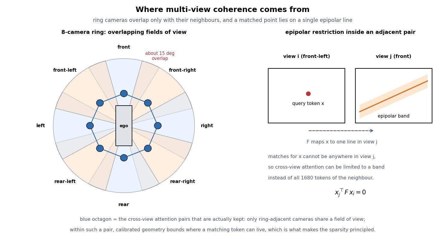
Left panel: top-down view of a vehicle with eight camera field-of-view wedges arranged in a ring, labelled front, front-right, right, rear-right, rear, rear-left, left, and front-left, with a 15 degree overlap marked between neighbours and an octagon of lines connecting adjacent camera nodes to show which pairs exchange cross-view attention. Right panel: two image-plane rectangles for view i and view j, a marked point x in view i and the corresponding epipolar band drawn as a shaded stripe in view j, with the constraint that a matching token lies on that single line.

Figure 2: Coherence is a geometry problem before it is a modelling problem. Only ring-adjacent pairs share a field of view, and within a pair the epipolar constraint bounds where a matching token can live, so both the sparsity pattern and the conditioning signal are dictated by the calibrated rig.

Mathematical Formulation:
$z \in \mathbb{R}^{V \times T \times N \times c}$
$N = (H/p)(W/p) = 28 \times 60 = 1680$
$L = V T N = 8 \times 16 \times 1680 = 215040$
$\mathcal{L}(\theta) = \mathbb{E}\left[\lVert \epsilon - \epsilon_{\theta}(z_t, t, c) \rVert^2\right]$
$c = (r, a, b, z_{\mathrm{ctx}})$
$r_{uv} = (d_{uv},\ o \times d_{uv}) \in \mathbb{R}^{6}$

Where:

$z$ is the joint latent tensor being denoised, with $V=8$ views, $T$ latent frames, $N$ tokens per view-frame, and $c$ latent channels.
$H \times W = 448 \times 960$ is the per-view pixel resolution and $p = 16$ the combined tokenizer and patch downsampling factor, giving a $28 \times 60$ latent map.
$L$ is the total sequence length if the clip were flattened, the number that decides whether full attention is affordable.
$\epsilon$ is the sampled noise, $z_t$ the noised latent at level $t$ , and $\epsilon_{\theta}$ the diffusion transformer.
$c$ bundles the conditioning: per-view rays $r$ , ego action $a$ (speed and curvature), agent and map layout $b$ , and the overlapping context latents $z_{\mathrm{ctx}}$ from the previous window.
$r_{uv}$ is the Plücker embedding of the ray through pixel $(u,v)$ , with unit direction $d_{uv}$ and camera origin $o$ , so extrinsics and intrinsics enter as a 6-channel image instead of a flat vector.

Attention Cost Per Block:
$C_{\mathrm{full}} = L^2 = 4.62 \times 10^{10}$
$C_{\mathrm{spa}} = V T N^2 = 3.61 \times 10^{8}$
$C_{\mathrm{view}} = T N V^2 = 1.72 \times 10^{6}$
$C_{\mathrm{tmp}} = V N T^2 = 3.44 \times 10^{6}$
$C_{\mathrm{spa}} + C_{\mathrm{view}} + C_{\mathrm{tmp}} = 3.66 \times 10^{8}$

Factorization therefore costs about 0.8% of full joint attention at this shape, and almost all of the remaining cost is ordinary within-frame spatial attention. The cross-view and temporal axes together add under 1.5% on top of the spatial term, which is the practical reason multi-view coherence is affordable at all: the expensive part of the model is generating each image, not keeping the images consistent.

Log-scale line chart of attention pairs per transformer block against the number of camera views from 1 to 8, with 16 latent frames and 1680 tokens per view-frame. The full joint 4D attention curve rises quadratically from about 7.2e8 to 4.62e10 pairs, while the factorized spatial plus cross-view plus temporal curve rises nearly linearly from about 2.9e7 to 3.66e8 pairs, an annotation noting the roughly 126x gap at eight views.

Figure 3: Full joint attention over the flattened clip grows as $V^2$ while the factorized form grows close to linearly in $V$ , so the gap widens with every camera added to the rig. Adding a ninth or tenth view is a routine cost in the factorized design and prohibitive in the joint one.

Property	Independent per-view generation	Factorized view + time attention	Full joint 4D attention
Attention pairs per block	3.61e8 (spatial only)	3.66e8, about 1.4% overhead	4.62e10, roughly 126x more
Overlap agreement	None; only the shared layout condition, so seams disagree	Enforced on ring-adjacent pairs, optionally epipolar-banded	Enforced globally, mostly on pairs that never overlap
Temporal behaviour	Per-view only; the eight views desynchronize over rollout	Temporal axis plus one shared action keeps views in lockstep	Strongest in principle, but memory caps the clip length
Failure signature	Objects appear in one camera and vanish in its neighbour	Slow drift of far-field content and appearance across rollout	Out-of-memory or a clip too short to be useful for simulation
Practical verdict	Useless for BEV or occupancy training data	The production choice for ring-camera world models	Research ablation at small resolution or few frames

August 18, 2026

DL0127 DDPM Training Objective

What is the DDPM training objective, and why do we train the network to predict the noise rather than the clean image directly?

Answer

A denoising diffusion probabilistic model is trained by maximizing a variational bound on the data log-likelihood, and because both the forward corruption and the reverse posterior are Gaussian, that bound collapses into a sum of KL divergences whose only learnable content is a mean-matching term at each noise level. Reparameterizing that mean through the closed-form forward marginal turns every term into a weighted squared error between the injected noise $\epsilon$ and a network prediction, and Ho et al. then drop the per-step weight $\lambda_t$ to get the simple objective $L_{\mathrm{simple}} = \mathbb{E}\|\epsilon - \epsilon_\theta(x_t,t)\|^2$ . Predicting the noise is not a different model from predicting the clean image: $\epsilon$ -prediction, $x_0$ -prediction, and direct mean prediction are affine reparameterizations of one another given $x_t$ and $t$ , so they define the same optimum but different implicit loss weightings and different numerical conditioning. The practical reasons to regress noise are that the target is always unit-variance no matter how noisy the input is, that the residual structure lets the network pass the low-frequency content through instead of re-synthesizing it, and that discarding $\lambda_t$ under this parameterization down-weights the easy low-noise steps by roughly an order of magnitude, which empirically buys much better FID. It also makes the network a rescaled score estimator, which is what connects DDPM to score matching and to every ODE and SDE sampler built on top of it.

(1) The Objective Is One Scalar MSE: sample $x_0$ , sample $t \sim \mathcal{U}\{1,\ldots,T\}$ and $\epsilon \sim \mathcal{N}(0,I)$ , form $x_t$ in closed form, and regress $\epsilon$ . No per-step model, no adversarial term, no sequential rollout during training.
(2) It Comes From The ELBO, Not From Heuristics: each $L_{t-1}$ is a Gaussian KL whose learnable part is a mean difference, and substituting the forward marginal converts it into $\lambda_t\|\epsilon-\epsilon_\theta\|^2$ .
(3) Dropping $\lambda_t$ Is A Reweighting Choice: $\lambda_t$ is largest at small $t$ , so setting all weights to 1 shifts capacity toward the high-noise steps that decide global structure.
(4) The Target Is Scale-Stable: $\epsilon$ is standard normal for every $t$ , so a single output head with fixed normalization works across the whole schedule, whereas the difficulty of predicting $x_0$ varies enormously with $t$ .
(5) Residual Prediction Is Easier For A U-Net: at low noise, most of $x_t$ is already the answer, so predicting the small perturbation avoids forcing the network to reconstruct an image it was handed.
(6) Conditioning Flips At The Two Ends: converting $\epsilon_\theta$ to $\hat x_0$ amplifies error by $1/\sqrt{\mathrm{SNR}_t}$ , which is tiny at low noise and roughly 150x at $t=T$ , the reason v-prediction exists.

Left-to-right flow diagram of one DDPM training step: sample a clean image, sample a timestep and Gaussian noise, form the corrupted sample in closed form, pass it through the U-Net to predict the noise, compute the squared error against the sampled noise, and a dashed feedback arrow carrying the gradient step back to the U-Net

Figure 1: One training step. The closed-form forward marginal means an arbitrary timestep can be sampled directly, so training never simulates the chain; the loss is a single unit-variance regression shared by all $T$ noise levels.

The reweighting argument is the one that most candidates miss. Under the ELBO, the term at $t=1$ carries roughly 50x the weight of the term at $t=T$ for the standard linear schedule, and those low- $t$ terms correspond to removing almost imperceptible noise, a task that contributes little to perceptual quality but a lot to likelihood. Setting every weight to 1 in $\epsilon$ -space is therefore a deliberate trade of likelihood for sample quality, and it is why DDPM reports strong FID with mediocre bits-per-dimension. The conditioning argument cuts the other way at high noise: since $\hat x_0$ is recovered by dividing by $\sqrt{\bar\alpha_t}$ , a small noise error becomes a large image error near $t=T$ , so pure $\epsilon$ -prediction is a poor target for few-step or distilled samplers that must produce a usable $\hat x_0$ from the very first step. Finally, the identity $\epsilon_\theta = -\sqrt{1-\bar\alpha_t}\,s_\theta$ shows the trained network is a scaled score function, which is exactly what a probability-flow ODE or an annealed Langevin sampler needs, so the same checkpoint serves DDPM, DDIM, and higher-order solvers.

Mathematical Formulation:
$x_t = \sqrt{\bar\alpha_t}\,x_0 + \sqrt{1-\bar\alpha_t}\,\epsilon$
$L_{t-1} = \lambda_t\,\|\epsilon - \epsilon_\theta(x_t,t)\|^2$
$\lambda_t = \frac{\beta_t^2}{2\sigma_t^2\alpha_t(1-\bar\alpha_t)}$
$L_{\mathrm{simple}} = \mathbb{E}\left[\|\epsilon - \epsilon_\theta(x_t,t)\|^2\right]$
$\hat x_0 = \frac{x_t - \sqrt{1-\bar\alpha_t}\,\epsilon_\theta}{\sqrt{\bar\alpha_t}}$
$\epsilon_\theta(x_t,t) = -\sqrt{1-\bar\alpha_t}\,s_\theta(x_t,t)$

Where:

$x_0$ is a clean training sample, $x_t$ its corrupted version at step $t$ , and $\epsilon \sim \mathcal{N}(0,I)$ the injected noise that serves as the regression target.
$t \in \{1,\ldots,T\}$ is sampled uniformly, $\beta_t$ is the schedule, $\alpha_t = 1-\beta_t$ , and $\bar\alpha_t = \prod_{s=1}^{t}\alpha_s$ gives the closed-form marginal that makes single-step training possible.
$\epsilon_\theta$ is the U-Net with parameters $\theta$ , conditioned on $t$ through a sinusoidal timestep embedding.
$\lambda_t$ is the ELBO weight and $\sigma_t^2$ the reverse-process variance (commonly $\sigma_t^2 = \beta_t$ ); $L_{\mathrm{simple}}$ is $L_{t-1}$ with $\lambda_t$ replaced by 1.
$\mathrm{SNR}_t = \bar\alpha_t/(1-\bar\alpha_t)$ is the signal-to-noise ratio, which decreases monotonically in $t$ and sets the error amplification $1/\sqrt{\mathrm{SNR}_t}$ from noise space into image space.
$s_\theta(x_t,t) \approx \nabla_{x_t}\log q(x_t)$ is the score, so a trained $\epsilon_\theta$ doubles as a score model for ODE and SDE samplers.

Two-panel chart: left panel plots the ELBO per-step weight relative to its value at the final timestep on a log axis against the diffusion step, showing roughly fifty times more weight at small t than at large t, next to the flat unit weight used by the simple objective; right panel plots on a log axis the factor by which a prediction error is amplified into clean-image space for noise prediction, clean-image prediction, and v-prediction, with noise prediction rising from about 0.01 to about 150

Figure 2: The two quantitative reasons the parameterization matters. Left: dropping $\lambda_t$ removes a roughly 50x preference for the easiest low-noise steps. Right: the same trained error costs almost nothing in image space at low noise but is amplified by $1/\sqrt{\mathrm{SNR}_t}$ near $t=T$ , which is where v-prediction stays bounded.

Property	Noise prediction (DDPM)	Clean-image prediction	v-prediction
Target	The sampled noise, standard normal at every t	The data sample itself, with data-dependent statistics	A schedule-dependent mix of noise and data
Implicit weighting under uniform MSE	Down-weights low-noise steps, favors perceptual quality over likelihood	Up-weights low-noise steps by the SNR, closer to the raw ELBO	Roughly balanced across the schedule, close to SNR-plus-one weighting
Numerical weak spot	Error into image space amplified by about 150x near t = T	Error into noise space amplified near t = 0, where the residual is tiny	Amplification stays at or below 1 in both directions
Typical use	Pixel and latent diffusion with many sampling steps, Stable Diffusion 1.x and 2.0-base	Very short schedules, consistency-style objectives, some latent decoders	Progressive distillation, high-resolution and upscaling models, SD 2.1-v

August 17, 2026

DL0126 Contrastive Learning Pairs

What is contrastive learning, and what are positive and negative pairs?

Answer

Contrastive learning trains an encoder by comparison instead of by prediction of a label: it pulls the embeddings of things that should mean the same thing together and pushes everything else apart. A positive pair is two views of the same underlying content (two augmentations of one photo in SimCLR, an image and its caption in CLIP, two nearby audio segments in CPC), and a negative pair is an anchor paired with content assumed to be different (any other item in the batch). The standard objective, InfoNCE, turns this into a softmax classification problem: given an anchor, identify its single positive among one positive and $K$ negatives, using scaled cosine similarity as the logit. Positives define what the representation should be invariant to, and negatives are what prevents the trivial solution where the encoder maps every input to the same vector, a failure called representational collapse. The whole design problem of a contrastive system is therefore the pair-construction policy: a positive that is too easy teaches nothing, and a negative that is secretly a positive actively teaches the wrong thing.

(1) Positives Encode The Invariance You Want: whatever transformation you apply to build a positive pair is exactly the factor the encoder learns to discard, so color jitter buys color invariance and destroys any task where color is the signal.
(2) Negatives Are The Anti-Collapse Term: without a repulsive term the constant map $f(x) = c$ is a global minimum of the attraction loss, so negatives provide the uniformity pressure that spreads embeddings over the hypersphere.
(3) InfoNCE Is A $K+1$ -Way Classification: one positive logit in the numerator, the positive plus all negatives in the denominator, which is why the loss is bounded below by $\log(K+1)$ under a random encoder.
(4) Temperature Sets Hard-Negative Focus: small $\tau$ (0.05 to 0.1 is typical) concentrates almost all repulsive gradient on the few most similar negatives, while large $\tau$ treats all negatives nearly equally.
(5) Negative Count Is A Systems Problem: SimCLR needs batch sizes of 4096 or more to get enough in-batch negatives, MoCo decouples them with a momentum-encoder queue, and CLIP trained with a 32768 global batch across many GPUs.
(6) False Negatives Are The Main Bias: in-batch negatives assume every other sample is semantically different, which is false on class-imbalanced or deduplicated-poorly data, and the loss then pushes apart items that should be close.

Pairs do not have to come from augmentation. The general recipe is: find a cheap source of known agreement and treat everything else as disagreement. Augmentation gives agreement between two crops of one image; multimodal alignment gives agreement between an image and the alt-text scraped alongside it; temporal or spatial context gives agreement between adjacent frames, patches, or sentences; and labels give agreement between any two samples of the same class, which is what SupCon exploits to allow many positives per anchor. The negatives are almost always just the rest of the batch, because sampling them explicitly is expensive and in-batch negatives come for free with the forward pass already computed.

Two-panel diagram: left panel shows one source image producing two augmented views labeled anchor and positive while two other images in the batch produce negative views; right panel shows the same points on a unit circle with an attraction arrow from anchor to positive and dashed repulsion arrows pushing the negatives away

Figure 1: Pair construction and its geometric effect. Each anchor has exactly one positive (the other view of the same source) and $2N-2$ negatives (all views of the other images in the batch); on the unit hypersphere the loss is a single attractive force toward the positive balanced against repulsive forces from every negative.

Mathematical Formulation:
$s(u,v) = \frac{u^\top v}{\|u\|\,\|v\|}$
$\ell_i = -\log \frac{\exp(s_{i,i^+}/\tau)}{\sum_{k \neq i} \exp(s_{i,k}/\tau)}$
$\mathcal{L} = \frac{1}{2N}\sum_{i=1}^{2N} \ell_i$
$I(u;v) \geq \log K - \mathcal{L}_{\mathrm{InfoNCE}}$

Where:

$s(u,v)$ is the cosine similarity used as the logit, computed on L2-normalized embeddings $u = f(v)$ produced by the encoder (and, in SimCLR, a discarded projection head).
$\ell_i$ is the per-anchor NT-Xent loss and $\mathcal{L}$ its average over all $2N$ views of an $N$ -image batch.
$i$ indexes the anchor view, $i^{+}$ its unique positive, and $k$ ranges over every other view, so the denominator holds 1 positive and $2N-2$ negatives.
$\tau > 0$ is the temperature; the gradient weight on negative $k$ is its softmax probability, so shrinking $\tau$ sharpens that distribution onto the hardest negatives.
$I(u;v)$ is the mutual information between the two views and $K$ the number of negatives, giving the standard InfoNCE lower bound: the bound saturates at $\log K$ , which is one reason large batches help.

Log-x line chart of the cumulative share of repulsive gradient carried by the hardest fraction of negatives, for temperature 0.05, 0.1 and 0.5 over 1024 negatives; the low-temperature curve rises almost vertically showing that the hardest one percent of negatives absorbs most of the gradient

Figure 2: Temperature decides which negatives matter. At $\tau = 0.05$ the hardest 1% of negatives absorbs most of the repulsive gradient, making training an implicit hard-negative miner that is also maximally sensitive to false negatives; at $\tau = 0.5$ the pressure is spread nearly uniformly and the embedding space stays smoother but less discriminative.

Aspect	Augmentation (SimCLR, MoCo)	Multimodal (CLIP, ALIGN)	Supervised (SupCon)
Anchor	One augmented view of an image	An image embedding	A labeled sample
Positive	A second augmentation of the same image (exactly one)	The paired caption text (exactly one, symmetric loss both directions)	Every other sample sharing the label (many per anchor)
Negatives	All 2N-2 other views, or a momentum queue of 65k stale keys	All other captions in the global batch (32k in CLIP)	Only samples with a different label, so false negatives vanish
Invariance learned	To the augmentation family you chose (crop, color, blur)	To modality and phrasing, giving a shared image-text space	To everything within a class, which can over-collapse fine detail
Main failure mode	Augmentation removes task-relevant signal; shortcut solutions from crop statistics	Noisy or generic captions produce weak positives; batch size dominates cost	Needs labels, so it is not self-supervised and inherits label noise

August 17, 2026