Tag: GenAI

DL0125 Action-Conditioned World Model

Explain the architecture of an Action-Conditioned World Model for autonomous driving, of the kind Wayve describes for its GAIA models.

Answer

An action-conditioned world model is a generative model of future sensor data whose predictions are explicitly steered by the ego vehicle’s own control commands, so it can answer “what would the road look like in three seconds if I brake at 5 m/s² instead of holding speed?”. Architecturally it factors into four blocks that are trained in two stages: a video encoder that compresses multi-camera frames into a small latent grid, an action and context encoder that embeds the low-dimensional control signal, a latent dynamics model that rolls the compressed state forward in time, and a decoder plus auxiliary heads that render latents back to pixels or BEV occupancy. Almost every production-scale system follows this shape and differs only in the dynamics block: GAIA-1 uses a 6.5B-parameter causal transformer over discrete video tokens with a separate diffusion video decoder, GAIA-2 replaces it with a flow-matching diffusion transformer over continuous latents so five surround views stay geometrically consistent, and Dreamer-style recurrent state-space models keep a compact deterministic-plus-stochastic state for reinforcement learning in imagination. The reason compression comes first is the same as in latent diffusion: at 6.25 Hz a 26-frame context of $288 \times 512$ frames is 3.8M pixels per frame-stack but only 14,976 latent tokens, and the dynamics model’s cost is quadratic in that number. What makes the model a simulator rather than a video generator is the rollout loop plus faithful action adherence, which is precisely where these models are weakest and where interviewers push.

(1) Observation Encoder: a VQ or KL-regularized video autoencoder with spatial factor $f = 16$ to $32$ maps each frame to an $18 \times 32$ grid; it is trained first with perceptual and adversarial losses, then frozen.
(2) Action And Context Conditioning: a 2-D action (curvature and acceleration) is embedded by a small MLP and injected per frame at every block, as prefix tokens or through AdaLN modulation, alongside text prompts, agent bounding boxes, and camera calibration.
(3) Latent Dynamics Backbone: a causal spacetime transformer predicting the next token, or a diffusion/flow-matching transformer denoising a whole latent chunk conditioned on the past; this is where nearly all parameters live.
(4) Decoder And Auxiliary Heads: a diffusion or convolutional decoder for video, plus cheap heads for BEV occupancy, collision cost, and value that planning actually consumes.
(5) Two-Stage Training With Teacher Forcing: the dynamics model always sees ground-truth latents during training, which creates the exposure-bias gap that dominates long-horizon rollouts.
(6) Three Consumers: closed-loop policy evaluation against counterfactual actions, planning or RL in imagination, and generation of rare corner-case scenarios that fleets rarely log.

Left to right pipeline: five surround cameras feed a video tokenizer producing an 18 by 32 latent per frame, a dynamics transformer conditioned on action, text, agent boxes and camera pose predicts future latents with an autoregressive rollout loop, and a decoder renders predicted video and BEV occupancy

Figure 1: The four blocks of an action-conditioned world model. Only the frozen codec ever touches pixels, the action modulates every block of the dynamics model, and the rollout loop is what turns a video generator into a driving simulator.

How the action enters is the part worth rehearsing. A two-number control signal has to influence a token stream dominated by appearance, so injecting it once at the input is not enough: it is embedded per frame and re-applied at every layer, and it must be time-aligned to the interval it causes rather than the frame it was logged with. Two failure modes follow directly. First, shortcut learning: logged actions are almost perfectly predictable from the visible road geometry, so a model can minimize training loss while ignoring $a_t$ entirely, and you only detect this by rolling out counterfactual actions that contradict the scene. Second, weak controllability at sampling time, which is why conditioning is dropped for 10-20% of training samples so that classifier-free guidance can later amplify action adherence. Evaluation therefore needs an action-following metric (does the rendered ego trajectory match the commanded one?) next to FID or FVD, because generative realism and control fidelity move independently.

Mathematical Formulation:
$z_t = \mathcal{E}(o_t)$
$h_t = f_\theta(h_{t-1}, z_{t-1}, a_{t-1})$
$\hat{z}_t \sim p_\theta(z_t \mid h_t, a_{t-1})$
$\hat{o}_t = \mathcal{D}(h_t, \hat{z}_t)$
$\mathcal{L} = \mathcal{L}_{\text{obs}} + \beta \, \mathcal{L}_{\text{dyn}}$
$\mathcal{L}_{\text{obs}} = -\log p_\theta(o_t \mid h_t, z_t)$
$\mathcal{L}_{\text{dyn}} = D_{KL}\!\left(q_\phi(z_t \mid h_t, o_t) \,\|\, p_\theta(z_t \mid h_t)\right)$
$p(z_{1:T} \mid a_{1:T}) = \prod_{t=1}^{T} p(z_t \mid z_{1:t-1}, a_{1:t-1})$
$N = T \cdot (H/f) \cdot (W/f)$
$N = 26 \cdot 18 \cdot 32 = 14{,}976$

Where:

$o_t$ is the multi-camera observation at step $t$ and $\hat{o}_t$ its prediction; $a_t$ is the ego action (curvature and acceleration, or steering and pedal).
$z_t$ is the compressed observation latent and $h_t$ the deterministic recurrent or attention-carried state that summarizes the past.
$\mathcal{E}$ and $\mathcal{D}$ are the frozen encoder and decoder, $f_\theta$ the dynamics backbone, $p_\theta$ the action-conditioned prior, and $q_\phi$ the posterior that also sees the true observation.
$\beta$ balances reconstruction against the dynamics (KL) term; in practice it is annealed and often free-bits clipped so the prior does not collapse onto the posterior.
$T$ is the context length in frames, $H \times W$ the frame resolution, $f$ the spatial compression factor, and $N$ the token count whose square drives attention cost.
Required initial conditions for a rollout: $h_0 = 0$ and a real context $z_{1:k}$ encoded from logged frames, after which only actions are supplied and $j > k$ steps are pure imagination.

Left panel: bird's-eye view of three ego trajectories branching from the same start under hold-speed, brake and lane-change action sequences, with a braking lead vehicle and a predicted collision marker. Right panel: prediction error versus rollout horizon for one-step re-encoding, free-running rollout, and a variant with action tokens ablated

Figure 2: Left: fixing the initial latent and varying only the action sequence produces counterfactual rollouts, the property that makes the model usable for closed-loop evaluation. Right: because training is teacher-forced, free-running error compounds superlinearly, and ablating the action tokens makes it worse still.

Dynamics block	Discrete-token autoregressive	Latent diffusion / flow matching	Recurrent state-space (RSSM)
Latent representation	VQ codebook indices, 576 tokens per frame	Continuous latent grid, tens of channels, temporally compressed	Small vector state: deterministic GRU plus categorical stochastic units
How the action enters	Per-frame prefix tokens in the causal sequence	AdaLN modulation or cross-attention at every block, with conditioning dropout	Concatenated into the recurrent transition at each step
Rollout cost	Hundreds of sequential token decodes per frame; slowest	Tens of denoising steps per chunk, parallel across positions	One cheap matrix step per frame; fast enough for RL in imagination
Strength	Exact likelihoods, easy long-context scaling, LLM tooling reuse	Best photorealism and multi-view consistency; controllable via guidance	Compact enough to train a policy on millions of imagined steps
Typical failure mode	Quantization artifacts and drift after a few seconds of rollout	Plausible but unfaithful scenes; ignores the action unless guided	Blurry reconstructions; posterior collapse hides rare agents
Representative system	GAIA-1	GAIA-2, Vista, NVIDIA Cosmos	DreamerV3, MILE

August 17, 2026

DL0122 V-JEPA vs Video World Models

Compare V-JEPA (Joint-Embedding Predictive Architecture) with video generation world models such as OpenAI’s Sora or NVIDIA Cosmos. What does each objective actually learn, and when would you deploy one over the other?

Answer

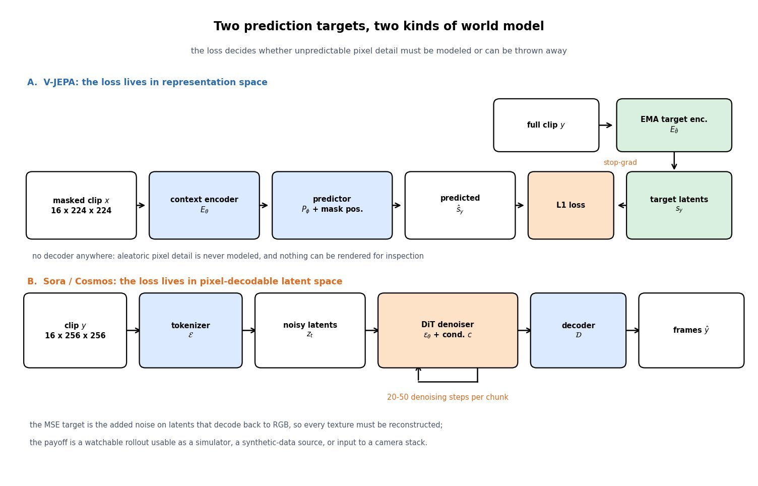
Both families are trained by predicting the unseen part of a video, and both are called world models, but they differ in where the prediction target lives. V-JEPA masks a large 3D region of a clip and trains a predictor to regress the embeddings of that region produced by an EMA target encoder, using an L1 loss in representation space; there is no decoder anywhere in the system, so the model is never asked to reproduce a pixel. Sora and Cosmos Predict instead train a generative model (a diffusion transformer over spacetime latent patches, or an autoregressive token model) to reconstruct the actual frames, which forces the network to spend capacity on every detail, including detail that is fundamentally unpredictable, such as the exact texture of foliage or the phase of a reflection. That single design choice cascades: V-JEPA gets a compact motion-aware representation and a rollout that costs one forward pass per step, which is what makes energy-based planning tractable, while generative world models get a renderable future that can serve as a simulator, a synthetic-data generator, or an input to an existing camera-based perception stack. Neither dominates; the question to ask in an interview is whether your downstream consumer is a policy or a pixel pipeline.

(1) Target Space: V-JEPA minimizes distance between predicted and EMA-encoded latents; Sora and Cosmos minimize a reconstruction or denoising loss defined on tokenizer latents that decode back to RGB.
(2) Discarded Information Is A Feature: because the target is learned, JEPA can drop aleatoric high-frequency detail instead of averaging over it, which is exactly what produced blurry futures in older pixel-space predictors.
(3) Collapse Risk: a learned target can be gamed by a constant function, so JEPA needs stop-gradient plus an EMA teacher and aggressive 3D block masking; a generative model has a fixed data target and cannot collapse.
(4) No Rendering: V-JEPA cannot show you its prediction, so debugging and human review happen through probes and downstream task metrics, not by watching a video.
(5) Rollout Cost: one predictor call per latent step versus tens of denoiser calls plus a decoder pass, a difference of one to two orders of magnitude inside a model-predictive control loop.
(6) Evaluation Protocol: JEPA is scored with frozen attentive probes on motion-heavy benchmarks and with planning success rate; generative world models are scored with FVD, human preference, physics-consistency suites, and sim2real transfer of policies trained on their output.

Two stacked architecture rows: V-JEPA encodes a masked clip, runs a predictor, and compares predicted latents against stop-gradient EMA target latents with an L1 loss; a video world model encodes a clip with a causal tokenizer, iterates a DiT denoiser for tens of steps, and decodes back to frames

Figure 1: The two families share a video encoder but differ in the prediction target: V-JEPA regresses EMA target embeddings and never instantiates a pixel, while a generative world model passes through a tokenizer, an iterative denoiser, and a decoder that must reconstruct every frame.

The masking strategy is what makes the latent objective non-trivial. V-JEPA masks large 3D blocks that span the full temporal extent of the clip, removing on the order of 90 percent of the tubelet tokens, so the predictor cannot solve the task by interpolating from neighboring patches and is pushed toward object identity, motion, and rough physics. V-JEPA 2 scaled this recipe to a ViT-g encoder over more than a million hours of internet video and then post-trained an action-conditioned predictor on roughly 62 hours of unlabeled robot video, after which planning is just a search over action sequences whose predicted latent lands closest to a goal image embedding. Cosmos takes the opposite bet at similar scale, curating on the order of tens of millions of hours of video into diffusion and autoregressive world foundation models plus tokenizers, precisely because a physical-AI developer wants renderable, controllable rollouts they can feed into an existing autonomy stack. The two are complementary in practice: Cosmos ships a separate reasoning model alongside its generators, and several robotics stacks now use a generative model for data augmentation and a latent predictor for the control loop.

Mathematical Formulation:
$s_y = E_{\bar{\theta}}(y)$
$\hat{s}_y = P_{\phi}(E_{\theta}(x), m)$
$\mathcal{L}_{\mathrm{JEPA}} = \lVert \hat{s}_y - \mathrm{sg}(s_y) \rVert_1$
$\bar{\theta} \leftarrow \tau \bar{\theta} + (1 - \tau)\,\theta$
$\mathcal{L}_{\mathrm{gen}} = \mathbb{E}\left[\lVert \epsilon - \epsilon_{\theta}(z_t, t, c) \rVert_2^2\right]$
$a^{*} = \arg\min_{a} \lVert P_{\phi}(s_t, a) - s_g \rVert_1$

Where:

$x$ is the visible (context) part of a clip and $y$ the masked target region; $m$ carries the positional mask tokens telling the predictor where to predict.
$E_{\theta}$ is the online encoder, $E_{\bar{\theta}}$ the EMA target encoder, and $P_{\phi}$ the narrow predictor discarded after pretraining.
$\mathrm{sg}(\cdot)$ is the stop-gradient that blocks the trivial solution, and $\tau$ is the EMA momentum, typically ramped from about 0.998 toward 1.
$z_t$ is the noised tokenizer latent at diffusion step $t$ , $\epsilon$ the sampled Gaussian noise, $\epsilon_{\theta}$ the denoiser, and $c$ the conditioning (text, past frames, or actions).
$s_t$ is the current latent state, $a$ a candidate action sequence, and $s_g$ the goal embedding; the planner requires an initial condition $s_t = E_{\theta}(o_t)$ from the current observation.

Log-scale bar chart of forward passes per planning step for a 200-candidate 16-step CEM search: 3200 for a one-pass latent predictor, 12800 for a distilled four-step video diffusion model, and 96000 for a thirty-step video diffusion world model

Figure 2: For the same 200-candidate, 16-step CEM search, a single-pass latent predictor needs 3,200 network calls while a 30-step generative rollout needs 96,000, before the decoder is even invoked; this 30x gap is why planning loops favor latent prediction.

Property	V-JEPA (latent predictive)	Sora / Cosmos (generative world model)
Training target	Embeddings from an EMA copy of the encoder, L1 loss	Noise or next token on VAE latents that decode to RGB
Handles stochastic detail by	Dropping it from the representation	Sampling it, which costs capacity and steps
Can render a future	No decoder; futures exist only as vectors	Yes, watchable and consumable by any vision stack
Cost per rollout step	One predictor forward pass	Tens of denoiser passes plus a decode
Main pathology	Representation collapse and shortcut solutions under weak masking	Physically implausible but photoreal rollouts, plus error accumulation over long horizons
Natural deployment	Frozen backbone for recognition and anticipation; goal-conditioned planning	Synthetic data, neural simulators, scenario replay, content generation

August 17, 2026

DL0111 SigLIP vs CLIP

What are the differences between SigLIP and CLIP?

Answer

CLIP and SigLIP share the same dual-encoder architecture, the same cosine-similarity scoring, and the same zero-shot classification recipe; the substantive difference is the training objective. CLIP optimizes a softmax InfoNCE loss in which each image’s logit row is normalized over every text in the batch and each text’s column over every image, so the loss contribution of a single pair depends on the entire batch, and the distributed implementation needs an all-gather plus a global normalization pass. SigLIP replaces this with a pairwise sigmoid loss that treats each of the $N^2$ cells of the similarity matrix as an independent binary decision (“is this a real pair?”), using a shared learnable temperature plus a learnable bias $b$ initialized to $-10$ to absorb the fact that only $N$ of the $N^2$ pairs are positive. Because nothing is normalized across the batch, the loss decomposes into $b \times b$ blocks, which lets SigLIP be implemented as a memory-efficient ring over devices and trained at batch sizes a softmax implementation cannot fit. Empirically the sigmoid loss is clearly better at small and moderate batch sizes, the two objectives converge above roughly 32k examples per step, and the million-example batch study SigLIP made possible showed that accuracy saturates long before that. That efficiency, plus the shape-optimized SoViT-400m/14 backbone released with it, is why SigLIP checkpoints became the default vision tower in many recent vision-language models such as PaliGemma.

(1) Loss Form: CLIP uses two symmetric softmax cross-entropies over the batch; SigLIP uses one binary logistic loss per pair, summed over the full $N \times N$ grid.
(2) Batch Coupling: softmax logits are only meaningful after a global normalization, so every device must see all $2N$ embeddings; sigmoid logits are independent, so blocks can be scored and reduced locally.
(3) Extra Bias Parameter: the sigmoid objective faces an extreme $N^2 - N$ negatives against $N$ positives imbalance, which the learnable bias fixes by starting every logit near “not a pair”.
(4) Batch-Size Behavior: sigmoid wins at 4k to 16k, matches softmax above roughly 32k, and both saturate rather than improving toward one million.
(5) Everything Else Is Unchanged: image tower, text tower, unit-norm embeddings, and prompt-based zero-shot evaluation are identical, so SigLIP is effectively a drop-in replacement at the loss layer.
(6) Practical Differences In The Checkpoints: public English SigLIP models use a 32k SentencePiece vocabulary with a 64-token text context (the original paper’s initial experiments used 16, but the released checkpoints increased it to 64), shorter than CLIP’s 77-token BPE context, which matters when captions are long.

Two 4 by 4 image-text similarity matrices. On the left, arrows show softmax normalization along every row and every column, coupling all pairs. On the right, each cell is an independent binary label scored by a sigmoid with learnable temperature and bias.

Figure 1: Both objectives see the same similarity matrix. CLIP normalizes each row and column, so a single logit’s gradient depends on the whole batch; SigLIP scores each cell as an independent binary label with a shared temperature and bias, which removes the coupling entirely.

Mathematical Formulation:
$s_{ij} = t\, x_i^{\top} y_j$
$\mathcal{L}_{\mathrm{i2t}} = -\frac{1}{N}\sum_{i} \log \frac{e^{s_{ii}}}{\sum_{j} e^{s_{ij}}}$
$\mathcal{L}_{\mathrm{t2i}} = -\frac{1}{N}\sum_{j} \log \frac{e^{s_{jj}}}{\sum_{i} e^{s_{ij}}}$
$\mathcal{L}_{\mathrm{CLIP}} = \tfrac{1}{2}\left(\mathcal{L}_{\mathrm{i2t}} + \mathcal{L}_{\mathrm{t2i}}\right)$
$\mathcal{L}_{\mathrm{SigLIP}} = \frac{1}{N}\sum_{i}\sum_{j}\log\left(1 + e^{-z_{ij}(s_{ij} + b)}\right)$

Where:

$x_i$ and $y_j$ are the unit-norm image and text embeddings, so $x_i^{\top} y_j$ is a cosine similarity in $[-1, 1]$ .
$s_{ij}$ is the scaled logit and $t = \exp(t')$ is the learnable temperature, parameterized in log space in both methods.
$i, j \in \{1, \ldots, N\}$ index the global batch; the diagonal $i = j$ holds the $N$ true pairs and the off-diagonal holds $N^2 - N$ negatives.
$z_{ij} = +1$ for a matched pair and $z_{ij} = -1$ otherwise, which is the binary label the sigmoid loss regresses on.
$b$ is the learnable bias unique to SigLIP, with the required initialization $b = -10$ and $t' = \log 10$ ; CLIP has no analogue because its softmax is shift-invariant.

The engineering consequence is the part interviewers usually probe. In a softmax implementation the batch is a single indivisible unit: after the all-gather each of the $D$ devices holds all $2N$ embeddings and materializes an $N \times b$ logit slab, and the row and column sums must be reduced across devices before any gradient exists. SigLIP instead keeps each device’s image chunk local and passes text chunks around a ring, accumulating loss from one $b \times b$ block at a time, so peak logit memory drops by a factor of $D$ and no cross-device normalization is needed. This is exactly what allowed the authors to sweep batch size up to one million and demonstrate saturation, and it is also why the SigLiT variant, which locks a pretrained image tower and trains only the text side, reached 84.5% ImageNet zero-shot accuracy in two days on four TPUv4 chips. The trade-off is two extra hyperparameters to get right: a badly initialized bias makes the first thousands of steps a wasted fight against the negative-pair prior.

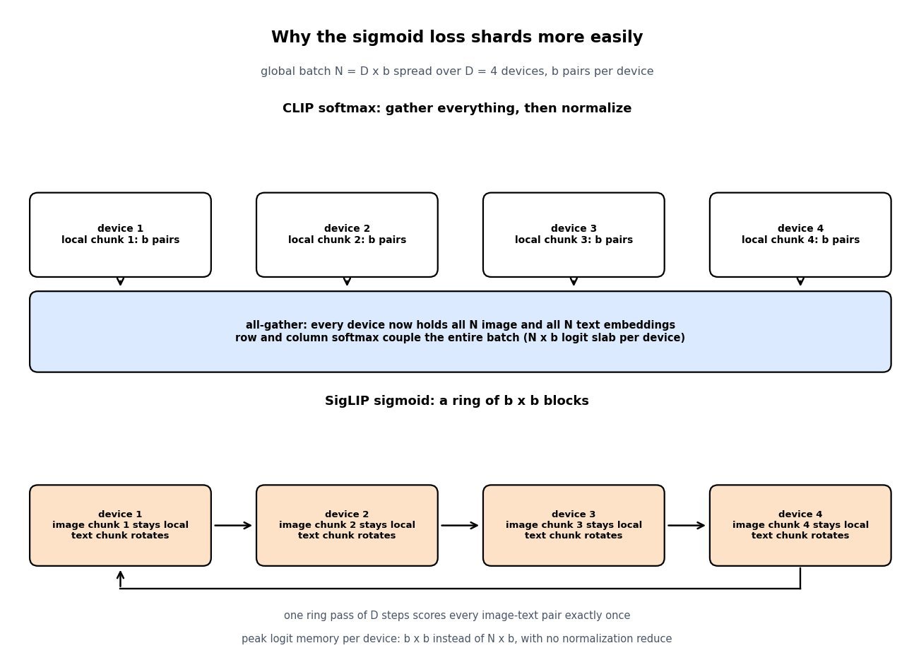
Top panel: four devices each holding a local chunk feed into an all-gather box where every device holds all N embeddings for a global softmax. Bottom panel: four devices keep their image chunk local while text chunks rotate around a ring, scoring one b by b block per step.

Figure 2: The softmax loss forces an all-gather and a global normalization, so each device carries an $N \times b$ logit slab. The sigmoid loss decomposes, so a ring of $D$ steps covers every pair while only $b \times b$ logits exist at once.

Property	SigLIP (sigmoid loss)	CLIP (softmax InfoNCE)
Objective	One binary logistic loss per image-text pair over the full grid	Two symmetric cross-entropies over row-wise and column-wise softmax
Batch coupling	None; the loss is a sum of independent terms	Global; every logit is normalized against the whole batch
Extra parameters	Learnable temperature plus a learnable bias, initialized to log 10 and -10	Learnable temperature only; a bias would cancel in the softmax
Distributed cost	Chunked ring; peak logit memory b x b per device, no normalization reduce	All-gather of all embeddings plus an N x b logit slab per device
Small batch (4k to 16k)	Clearly stronger zero-shot accuracy at equal examples seen	Degrades noticeably; the normalization has few negatives to work with
Very large batch	Feasible up to one million, but accuracy saturates near 32k	Comparable above roughly 32k, but memory-bound before that
Text context	64 tokens (16 in the original paper), 32k SentencePiece in the English releases	77 tokens, 49k byte-pair vocabulary
Typical role today	Default frozen vision tower for many VLMs, notably SoViT-400m/14	Legacy ecosystem: diffusion text conditioning, CLIPScore, many distilled models

August 17, 2026

DL0106 Stable Diffusion Architecture

Explain the key components of the Stable Diffusion architecture and how they interact during image generation.

Answer

Stable Diffusion is three separately trained networks plus one training-free sampler, and only one of the three is trained on the diffusion objective. A frozen KL-regularized VAE maps a $512 \times 512 \times 3$ image to a $64 \times 64 \times 4$ latent and back; a frozen CLIP text encoder turns the prompt into a $77 \times 768$ sequence of token embeddings; and a conditional U-Net (860M parameters in SD 1.5) predicts the noise present in a noisy latent, given the timestep and the text context. At generation time the sampler starts from $z_T \sim \mathcal{N}(0, I)$ on the latent grid and repeats a fixed loop: call the U-Net, combine the conditional and unconditional predictions with classifier-free guidance, then let the scheduler (DDIM, Euler, DPM-Solver) take one step of the reverse process. After 20 to 50 such steps the VAE decoder is called exactly once to turn the final latent into pixels, so the full path is encode → denoise → decode with the text encoder feeding every denoising step through cross-attention.

(1) VAE Codec: a convolutional encoder and decoder pair, frozen after stage-one training with an L1 plus LPIPS plus patch-GAN objective, that removes imperceptible high-frequency detail so the denoiser works on 16,384 values instead of 786,432.
(2) Text Encoder: CLIP ViT-L/14’s transformer, frozen, producing per-token hidden states rather than a single pooled vector, which is what makes word-level prompt control possible.
(3) U-Net Denoiser: the only trained diffusion component, built from ResBlocks that receive a sinusoidal timestep embedding through a learned projection added to their feature maps, interleaved with transformer blocks.
(4) Cross-Attention Is The Conditioning Interface: queries come from the latent feature map, keys and values come from the text context, so the prompt influences the image at 16 separate points in SD 1.5’s U-Net.
(5) Scheduler: not a network at all but a numerical solver for the reverse SDE or probability-flow ODE, which is why you can swap samplers and step counts on a trained checkpoint without retraining.
(6) Classifier-Free Guidance: each step runs the U-Net twice, once with the prompt and once with the empty string, and extrapolates between them, which doubles the per-step cost and is the main knob for prompt adherence.

Block diagram of Stable Diffusion generation: a text prompt enters a frozen CLIP text encoder producing a 77 by 768 context that feeds cross-attention in the U-Net denoiser; starting from Gaussian noise in a 64 by 64 by 4 latent, the U-Net output passes through classifier-free guidance and a scheduler step, loops for 20 to 50 steps, and the final latent is decoded once by the frozen VAE decoder into a 512 by 512 image

Figure 1: The loop is the architecture. The U-Net is evaluated twice per step for guidance, the text encoder runs once for the whole generation, and the decoder runs once at the end; everything inside the loop stays on the small latent grid.

Inside the U-Net the latent descends a resolution ladder, $64 \rightarrow 32 \rightarrow 16 \rightarrow 8$ , with channel widths 320, 640, 1280, 1280, and climbs back up with skip concatenations from the matching encoder level. Attention is deliberately not applied everywhere: in SD 1.5 the transformer blocks sit at the $64$ , $32$ , and $16$ levels plus the mid block, and the deepest $8 \times 8$ level is pure convolution, because self-attention cost grows as $O(N^2)$ in the token count and the highest-resolution level already carries 4,096 tokens. SDXL rebalances exactly this: it drops attention at the finest level entirely and stacks far more transformer blocks at $32$ and $16$ , which is how it reaches 2.6B parameters while remaining trainable at $1024 \times 1024$ . Each transformer block is self-attention, then cross-attention, then a GEGLU feed-forward, so spatial coherence and prompt alignment are handled by two different mechanisms in the same block.

U-shaped diagram of the SD 1.5 denoiser: four downsampling levels at 64 by 64 with 320 channels, 32 by 32 with 640, 16 by 16 with 1280 and 8 by 8 with 1280, a mid block with attention, and four upsampling levels, with dashed skip-concatenation links between matching levels and attention marked at the top three levels and the mid block only

Figure 2: The SD 1.5 U-Net applies self-attention and cross-attention at three of four resolutions and leaves the deepest $8 \times 8$ level convolution-only; skip concatenations carry high-frequency structure past the bottleneck so the decoder path can restore fine detail.

Mathematical Formulation:
$z_T \sim \mathcal{N}(0, I)$
$Q = W_Q\,\varphi(z_t)$
$K = W_K\,\tau(y)$
$V = W_V\,\tau(y)$
$\mathrm{Attn} = \mathrm{softmax}\!\left(\frac{QK^{\top}}{\sqrt{d}}\right)V$
$\hat{\epsilon}_t = \epsilon_u + s\,(\epsilon_c - \epsilon_u)$
$z_{t-1} = \mathrm{Step}(z_t, \hat{\epsilon}_t, t)$
$\hat{x} = \mathcal{D}(z_0 / s_z)$

Where:

$z_t \in \mathbb{R}^{64 \times 64 \times 4}$ is the latent at timestep $t$ , and $\hat{x}$ is the decoded image.
$\varphi(z_t)$ is the flattened spatial feature map entering a transformer block, and $\tau(y)$ is the frozen CLIP context of shape $77 \times 768$ .
$W_Q, W_K, W_V$ are the per-layer projections and $d$ is the head dimension; queries carry image content while keys and values carry text.
$\epsilon_c = \epsilon_\theta(z_t, t, \tau(y))$ and $\epsilon_u = \epsilon_\theta(z_t, t, \tau(\varnothing))$ are the conditional and unconditional noise predictions, and $s$ is the guidance scale (typically $5 \leq s \leq 9$ ).
$\mathrm{Step}$ is the scheduler update (DDIM, Euler, DPM-Solver), applied for $t$ descending over the chosen 20 to 50 timesteps.
$\mathcal{D}$ is the frozen VAE decoder and $s_z = 0.18215$ the latent scaling constant; the required initial condition is $z_T \sim \mathcal{N}(0, I)$ , which only holds because $s_z$ normalizes the latent variance.

Component	SD 1.5	SDXL	SD3 / Flux
Latent codec	KL-VAE, f = 8, 4 channels, about 84M parameters	Retrained f = 8 VAE, still 4 channels	f = 8 VAE widened to 16 channels
Text encoder	CLIP ViT-L/14, 77 x 768 context	CLIP ViT-L plus OpenCLIP ViT-bigG, concatenated to 77 x 2048 plus a pooled vector	CLIP-L, CLIP-G and T5-XXL, giving long-prompt and typography understanding
Denoiser	U-Net, 860M, attention at 64, 32 and 16	U-Net, 2.6B, no attention at the finest level, deep transformer stacks at 32 and 16	MMDiT transformer, 2B to 12B, no convolutional U-Net at all
Conditioning path	Cross-attention in 16 transformer blocks	Cross-attention plus pooled text, original size and crop coordinates added to the timestep embedding	Joint self-attention over concatenated text and image tokens, with separate weights per modality
Objective and native resolution	Epsilon-prediction, 512 x 512	Epsilon-prediction base with a v-prediction refiner, 1024 x 1024	Rectified flow matching, 1024 x 1024 with multi-aspect buckets

August 17, 2026

DL0105 DiT: Diffusion Transformers

What is the core architectural innovation of Diffusion Transformers (DiT) compared to traditional U-Net-based diffusion models?

Answer

The core innovation is mostly subtractive: DiT deletes the multi-scale convolutional U-Net and replaces it with a plain ViT-style transformer that runs on a flat sequence of latent patch tokens at constant resolution and constant width, with no downsampling, no upsampling, and no encoder-decoder skip connections. A $32 \times 32 \times 4$ latent from an 8x VAE is cut into non-overlapping $p \times p$ patches ( $p = 2$ gives 256 tokens), linearly projected to width $d$ , given positional embeddings, and pushed through $N$ identical blocks. The only diffusion-specific machinery left is how conditioning enters: adaLN-Zero regresses a per-block scale, shift, and residual gate from the summed timestep and class embeddings, with the gate initialized to zero so each block starts as an identity map. Because the backbone is isotropic, sample quality becomes a smooth function of transformer Gflops rather than of hand-tuned channel schedules, and DiT-XL/2 (28 blocks, width 1152, 675M parameters, 118.6 Gflops) reached FID 2.27 with classifier-free guidance on ImageNet $256 \times 256$ after 7M training steps, ahead of the U-Net LDM and ADM baselines. That predictable scaling, plus the ability to reuse ordinary transformer infrastructure, is why later systems such as Stable Diffusion 3 and video generators adopted DiT-style backbones.

(1) Isotropic Token Stack: patchify once, then keep the sequence length and hidden width fixed through every block, so there is no multi-scale hierarchy and no skip connections to carry high-frequency detail.
(2) adaLN-Zero Conditioning: timestep and class are injected by modulating LayerNorm and gating the residual branch instead of through cross-attention or extra input channels, and the zero-initialized gate makes a 28-block stack start as the identity.
(3) Patch Size Is A Compute Knob: halving $p$ quadruples the token count and roughly quadruples backbone Gflops without adding parameters, which makes compute and capacity independently tunable.
(4) Quality Tracks Gflops: FID decreases monotonically with backbone Gflops across model sizes and patch sizes, so a smaller model with small patches can beat a larger model with large patches.
(5) Infrastructure Reuse: the backbone is a standard transformer, so FlashAttention, sequence and tensor parallelism, and spatiotemporal patching for video all transfer directly from the LLM and ViT ecosystem.

Side-by-side diagram: on the left a U-Net with three encoder ResBlocks descending in resolution, a mid block, three upsampling decoder blocks and dashed skip connections; on the right a DiT stack of patchify, 28 DiT blocks with adaLN-Zero conditioning, and a final linear unpatchify layer

Figure 1: The U-Net spends parameters on a resolution pyramid with skip connections, while DiT keeps one token sequence at fixed width and pushes all conditioning through adaLN-Zero modulation of each block.

The conditioning choice was not incidental. The DiT paper ablated four options at matched compute: in-context conditioning (append timestep and class as extra tokens), cross-attention to a two-token condition sequence, plain adaptive LayerNorm, and adaLN-Zero. The ranking was consistent, with adaLN-Zero best, then adaLN, then cross-attention, then in-context, and adaLN-Zero also added the fewest Gflops because it needs no extra tokens or extra attention operation. The zero-initialized gate matters because a deep residual stack whose blocks all start as identity behaves like a shallow network early in training, which is the same trick that stabilizes very deep ResNets and ViTs. The cost of dropping skip connections is that all high-frequency reconstruction has to be learned inside the token stack and by the VAE decoder, which is one reason DiT operates in a compressed latent space rather than on raw pixels.

Mathematical Formulation:
$T = \frac{H}{p} \cdot \frac{W}{p}$
$c = \mathrm{emb}(t) + \mathrm{emb}(y)$
$(\gamma_i, \beta_i, \alpha_i) = \mathrm{MLP}_i(c)$
$\hat{z} = (1 + \gamma_1)\,\mathrm{LN}(z) + \beta_1$
$z \leftarrow z + \alpha_1\,\mathrm{MSA}(\hat{z})$
$\mathcal{C}_{\mathrm{attn}} = O(T^2 d)$

Where:

$T$ is the token count after patchifying a latent of spatial size $H \times W$ with patch size $p$ ; for $H = W = 32$ and $p = 2$ this gives $T = 256$ .
$c$ is the pooled conditioning vector built from the diffusion timestep $t$ and the class or text embedding $y$ .
$\gamma_i, \beta_i$ are the scale and shift applied to the normalized activations of sub-layer $i$ , and $\alpha_i$ is the residual gate; $i \in \{1, 2\}$ indexes the attention and feed-forward sub-layers.
$z \in \mathbb{R}^{T \times d}$ is the token sequence, $\mathrm{LN}$ is LayerNorm without learnable affine parameters, and $\mathrm{MSA}$ is multi-head self-attention (the feed-forward sub-layer uses $\gamma_2, \beta_2, \alpha_2$ identically).
$\mathcal{C}_{\mathrm{attn}}$ is the per-layer attention cost, quadratic in $T$ and therefore quartic in the inverse patch size.
Required initial condition: $\alpha_1 = \alpha_2 = 0$ at step 0, so every block is an identity map and the residual stream passes through unchanged.

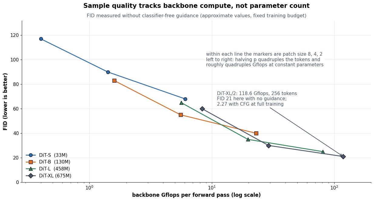
Log-x line chart of FID against backbone Gflops for DiT-S, DiT-B, DiT-L and DiT-XL, each line connecting patch sizes 8, 4 and 2, showing FID falling monotonically as Gflops rise

Figure 2: Approximate FID against backbone Gflops at a fixed 400K-step training budget and without classifier-free guidance, which is why the absolute values sit far above the guided FID 2.27 quoted for the fully trained DiT-XL/2. What matters here is the trend: quality tracks compute rather than parameter count, so DiT-B with $p = 2$ can outrun DiT-L with $p = 8$ despite having far fewer parameters.

Property	DiT	U-Net (ADM, LDM, SDXL)
Spatial handling	One fixed-length token sequence, no resampling and no skips	Resolution pyramid 32 → 16 → 8 → 4 → 8 → 16 → 32 with skip connections
Conditioning path	adaLN-Zero: per-block scale, shift, and zero-initialized residual gate from $c$	Timestep embedding added inside ResBlocks, text or class via cross-attention
Compute knobs	Depth, width, and patch size; patch size changes Gflops at constant parameters	Channel multipliers, blocks per level, and which levels get attention
Inductive bias	Minimal beyond positional embeddings, so it needs more data and compute to pay off	Strong locality and multi-scale bias, sample-efficient at small budgets
Cost as resolution grows	$O(T^2 d)$ attention, so latent compression and patch size are load-bearing	Convolutions grow linearly in pixels; attention only at low-resolution levels
Scaling behavior	FID a smooth decreasing function of Gflops, easy to extrapolate	Gains depend on hand-designed schedules and saturate less predictably

One caveat when quoting numbers in an interview: FID is only comparable within a fixed evaluation protocol. The headline 2.27 comes from the fully trained DiT-XL/2 sampled with classifier-free guidance at scale 1.5; the same checkpoint sampled without guidance lands near 9.6, and the scaling sweep above uses a much shorter 400K-step budget with no guidance at all. Guidance, training steps, sampler, and step count all move the number by more than the architectural gap being discussed, so state the protocol alongside the score.

August 16, 2026

DL0104 Score-Based Diffusion

What is the score-based / score-matching interpretation of diffusion models, as used in systems like Stable Diffusion?

Answer

The score-based view says a diffusion model never learns a density; it learns the score, the gradient of the log density $s(x) = \nabla_x \log p(x)$ . This is attractive because the gradient annihilates the intractable normalizing constant: if $p(x) = e^{-E(x)}/Z$ then $\nabla_x \log p(x) = -\nabla_x E(x)$ with no $Z$ anywhere, so an unnormalized energy model becomes trainable. Direct score matching still needs the intractable $\nabla_x \log p_{\text{data}}(x)$ , and the fix is denoising score matching: perturb the data with a known Gaussian kernel, and the score of the perturbed conditional is available in closed form, which reduces the loss to predicting the noise that was added. Because a single small noise level leaves the score undefined off the data manifold and unreliable in low-density regions, the model is trained over a continuum of noise levels, which turns into the forward SDE of Song et al. and makes sampling the simulation of a reverse-time SDE or its deterministic probability-flow ODE. The punchline is that DDPM’s noise-prediction network is the same object in different clothing: $s_\theta(x_t,t) = -\epsilon_\theta(x_t,t)/\sigma_t$ , so the discrete-time denoising story and the continuous-time score story are two parameterizations of one model.

(1) Model The Gradient, Not The Density: learning $\nabla_x \log p(x)$ removes the partition function, so the network output is an unconstrained vector field of the same shape as the data.
(2) Denoising Score Matching Makes It Tractable: Vincent’s identity shows that regressing onto $\nabla_{x_t}\log p(x_t \mid x_0)$ has the same minimizer as matching the true marginal score, and that target is just the scaled added noise.
(3) Multiple Noise Scales Are Essential: real data lies near a low-dimensional manifold where the score is ill-defined, and large noise levels smooth the density so the vector field is informative everywhere and connects separated modes.
(4) Sampling Is Numerical Integration: annealed Langevin dynamics, the reverse SDE, and the probability-flow ODE all consume only the learned score; the ODE additionally gives exact likelihoods and deterministic, invertible latents.
(5) Unifies VE And VP Diffusions: NCSN’s variance-exploding noise ladder and DDPM’s variance-preserving chain are two discretizations of the same SDE family, differing in $f$ , $g$ , and the loss weighting $\lambda_t$ .

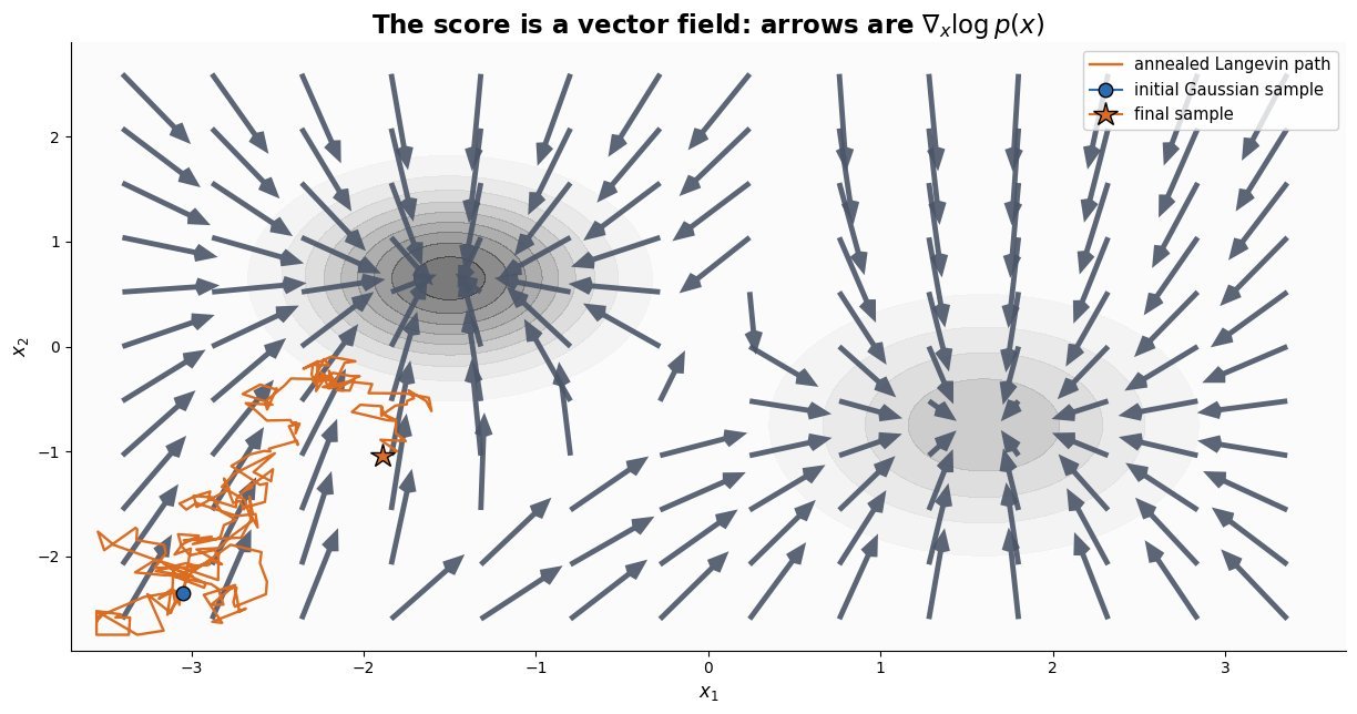
The geometric picture is worth holding onto. The score at a point is the direction of steepest increase in log density, so the learned field points from wherever you are toward nearby high-probability regions, and its magnitude grows as you move into the tails. Sampling then means dropping a Gaussian sample somewhere in space and following that field while injecting just enough noise to keep the chain from collapsing onto a single mode. The reason this needs annealing is that a score trained only at tiny noise is accurate on the data manifold and near-arbitrary far from it, where every initial sample actually starts.

Contour plot of a two-mode density with an overlaid arrow field pointing toward the modes, and a jagged Langevin sampling path starting in the empty lower-left corner and ending inside the left mode

Figure 1: The learned score is a vector field pointing toward high-density regions; a Langevin chain follows it from a random start and ends up distributed according to $p(x)$ , never evaluating the density itself.

Mathematical Formulation:
$s_\theta(x,t) \approx \nabla_x \log p_t(x)$
$x_t = \alpha_t x_0 + \sigma_t \epsilon$
$\nabla_{x_t} \log p(x_t \mid x_0) = -\frac{\epsilon}{\sigma_t}$
$\mathcal{L}(\theta) = \mathbb{E}\left[ \lambda_t \left\| s_\theta(x_t,t) + \frac{\epsilon}{\sigma_t} \right\|^2 \right]$
$dx = f(x,t)\,dt + g(t)\,dw$
$dx = \left[ f - g^2 s_\theta \right] dt + g\,d\bar{w}$
$dx = \left[ f - \tfrac{1}{2} g^2 s_\theta \right] dt$
$s_\theta(x_t,t) = -\frac{\epsilon_\theta(x_t,t)}{\sigma_t}$

Where:

$s_\theta(x,t)$ is the network output, a vector with the same shape as $x$ , approximating the score of the perturbed marginal $p_t$ .
$x_0$ is a clean data point, $x_t$ its noisy version, and $\epsilon \sim \mathcal{N}(0,I)$ the Gaussian draw.
$\alpha_t$ and $\sigma_t$ define the noise schedule; variance-preserving keeps $\alpha_t^2 + \sigma_t^2 = 1$ , variance-exploding fixes $\alpha_t = 1$ and grows $\sigma_t$ .
$t \in [0,T]$ indexes the noise level, with $p_T$ essentially pure Gaussian noise; $\lambda_t$ is the loss weighting, and the choice $\lambda_t = \sigma_t^2$ turns the objective into the plain noise-prediction MSE.
$f(x,t)$ is the drift and $g(t)$ the diffusion coefficient of the forward SDE; $w$ is a Wiener process and $\bar{w}$ its reverse-time counterpart, so the second SDE is integrated from $t = T$ down to $t = 0$ .
The final line is the reparameterization identity linking the score view to DDPM’s $\epsilon_\theta$ ; required initial condition for sampling: $x_T \sim \mathcal{N}(0, \sigma_T^2 I)$ for the VE case.

Three panels showing the same two-mode density smoothed by increasing Gaussian noise, with score arrows that are confined near the modes at small noise and fill the whole plane at large noise

Figure 2: Why a ladder of noise levels is required: at $\sigma = 0.05$ the score carries no usable signal away from the data, while at $\sigma = 1.5$ the smoothed field points inward from everywhere and bridges the two modes.

Property	Score SDE (VE, NCSN)	DDPM (VP, noise-pred)	Flow matching
Network output	Score, magnitude scales like 1/sigma_t	Unit-variance noise estimate	Velocity field of a probability path
Corruption	Add noise, variance grows to data scale	Shrink signal, keep total variance at 1	Straight interpolation between data and noise
Loss	Weighted denoising score matching	Same loss with weighting sigma_t squared	Regression onto the conditional velocity
Sampler	Annealed Langevin or predictor-corrector	Ancestral chain, or DDIM as an ODE	ODE solver on a near-straight path
Exact likelihood	Yes, via the probability-flow ODE	Only an ELBO in discrete time	Yes, continuous normalizing flow change of variables

August 16, 2026

DL0103 Stable Diffusion Latent Space

What is latent diffusion, and why does Stable Diffusion run diffusion in a VAE latent space?

Answer

Latent diffusion splits image generation into two stages that are trained separately: a convolutional autoencoder first compresses pixels into a small spatial latent, and the diffusion model then learns the noise process entirely inside that latent grid. Stable Diffusion uses a KL-regularized VAE with downsampling factor $f = 8$ , so a $512 \times 512 \times 3$ image becomes a $64 \times 64 \times 4$ latent: 786,432 values collapse to 16,384, a 48x reduction in the tensor the U-Net has to denoise. The motivation is that the two stages solve different problems. Pixel-space diffusion wastes most of its capacity and most of its training steps modeling imperceptible high-frequency detail, exactly the information a perceptual codec throws away for free; the autoencoder handles that perceptual compression once, and the diffusion model is left with the semantic compression problem of arranging layout, objects, and style. The compute argument is even stronger than the 48x suggests, because the U-Net contains self-attention: token count drops from 262,144 to 4,096, so any $O(N^2)$ attention block gets $f^4 = 4096$ times cheaper. That is what turned high-resolution text-to-image training from a large-cluster project into something reproducible on modest hardware, and what makes 50-step sampling on a consumer GPU feasible at all.

(1) Two-Stage Factorization: the autoencoder is trained first and then frozen; the diffusion model never sees a pixel, and the decoder is invoked exactly once at the end of sampling.
(2) Quadratic Savings On Attention: the latent grid has $f^2$ fewer positions, so convolutions get $f^2$ cheaper and self-attention gets roughly $f^4$ cheaper.
(3) It Is Not A Generative VAE: the KL weight is tiny (on the order of $10^{-6}$ ) and the reconstruction loss adds LPIPS plus a patch discriminator, so the encoder behaves as a sharp lossy codec rather than a prior you would ever sample from.
(4) Latent Scaling Matters: encoder outputs are multiplied by a constant (0.18215 for SD 1.x, 0.13025 for SDXL) so the latent has roughly unit variance and the standard noise schedule reaches a true $\mathcal{N}(0, I)$ terminal state.
(5) Cheap Conditioning And Editing: CLIP text embeddings enter through cross-attention at every latent resolution, and img2img, inpainting, and ControlNet all operate on the same small latent grid.
(6) The Decoder Is The Fidelity Ceiling: nothing the diffusion model does can recover detail the 4-channel latent discarded, which is why small text, fine textures, and tiny faces degrade first.

Pipeline diagram: a 512 by 512 by 3 image enters a VAE encoder producing a 64 by 64 by 4 latent, an iterative denoising U-Net conditioned by CLIP text cross-attention operates on the latent for T steps, and a VAE decoder maps the result back to pixels

Figure 1: Training and sampling both live in the 4,096-token latent grid; the frozen encoder and decoder are the only components that ever touch the 262,144-pixel image, and text conditioning enters the denoiser through cross-attention.

The choice of $f$ is a genuine trade-off rather than a free win. The original LDM ablations show that $f \in \{4, 8\}$ is the sweet spot: at $f = 1$ or $2$ training is slow because the model is still doing perceptual compression itself, while at $f = 32$ with only 4 channels the autoencoder becomes the bottleneck and sample quality saturates no matter how long the diffusion model trains. Channel count $c$ is the other lever, and it is the one that later models moved: SD3 and Flux keep $f = 8$ but raise the latent to 16 channels, quartering the compression ratio from 48 to 12 to trade a little step cost for a much better reconstruction ceiling on text and fine structure. A practical consequence of the frozen-codec design is that latents are model-specific: an SDXL latent decoded by an SD 1.5 decoder produces color-shifted garbage, because the two autoencoders were trained with different scaling and channel statistics.

Mathematical Formulation:
$z_0 = s \cdot \mathcal{E}(x)$
$\hat{x} = \mathcal{D}(z_0 / s)$
$z_t = \sqrt{\bar\alpha_t}\, z_0 + \sqrt{1 - \bar\alpha_t}\, \epsilon$
$\mathcal{L} = \mathbb{E}\left[\lVert \epsilon - \epsilon_\theta(z_t, t, \tau(y)) \rVert_2^2\right]$
$\rho = \frac{3 f^2}{c}$
$\rho = \frac{3 \cdot 64}{4} = 48$

Where:

$x \in \mathbb{R}^{H \times W \times 3}$ is the image and $\hat{x}$ its reconstruction; $z_0 \in \mathbb{R}^{h \times w \times c}$ is the clean latent with $h = H/f$ and $w = W/f$ .
$\mathcal{E}$ and $\mathcal{D}$ are the frozen VAE encoder and decoder, and $s$ is the latent scaling constant that normalizes the variance.
$t \in \{1, \ldots, T\}$ is the timestep, $\bar\alpha_t$ the cumulative noise schedule, and $\epsilon \sim \mathcal{N}(0, I)$ the sampled Gaussian noise.
$\epsilon_\theta$ is the latent denoiser (U-Net in SD 1.x and SDXL, a transformer in DiT-style successors), and $\tau(y)$ is the text-encoder output injected by cross-attention.
$f$ is the spatial downsampling factor and $c$ the latent channel count; $\rho$ is the element compression ratio, which is 48 for $f = 8, c = 4$ and 12 for $c = 16$ .
Required initial condition at sampling: $z_T \sim \mathcal{N}(0, I)$ on the latent grid, which only holds if $s$ was applied and $\bar\alpha_T \approx 0$ .

Log-scale bar chart of self-attention cost reduction relative to pixel space at 512 by 512 resolution: factor 1 for pixel space with 262144 tokens, 256 for f equals 4, 4096 for f equals 8, and 65536 for f equals 16

Figure 2: Because self-attention scales as $O(N^2)$ in the token count, compressing by $f$ cuts attention cost by $f^4$ ; the $f = 8$ setting used by Stable Diffusion buys a 4096x reduction while keeping the decoder’s reconstruction error acceptable.

Property	Latent diffusion (Stable Diffusion)	Single-stage pixel diffusion	Cascaded pixel diffusion
Where noise is added	A 64x64x4 VAE latent	Directly on RGB pixels at full resolution	Pixels at 64×64, then two super-resolution diffusion stages
Denoiser input size at 512×512	4,096 tokens, 16,384 values	262,144 tokens, 786,432 values	4,096 tokens in the base model, full resolution in the last upsampler
Training and sampling cost	Lowest; one model, attention roughly 4096x cheaper per block	Highest; attention is usually dropped or windowed to stay tractable	Moderate but multiplied by the number of stages
Fidelity ceiling	Bounded by decoder reconstruction error, independent of training length	No codec bottleneck; exact pixel modeling is possible	No codec bottleneck, but upsamplers can hallucinate detail
Typical failure mode	Mangled small text, smeared fine texture, artifacts on tiny faces	Under-trained global structure for a fixed compute budget	Error accumulation and train/test mismatch between stages

August 16, 2026

DL0102 Diffusion vs GAN vs VAE

Explain the fundamental principles of Diffusion Models, and compare their pros and cons with GANs, VAEs, and Flow-based models.

Answer

A diffusion model defines a fixed forward process that gradually corrupts data into Gaussian noise over $T$ steps, then learns the reverse process that removes a little noise at a time. The forward chain has no parameters and admits a closed form, so training reduces to a plain regression: sample a clean image $x_0$ , sample a timestep $t$ and noise $\epsilon$ , build the noisy state $x_t$ , and ask the network to predict $\epsilon$ . This denoising objective is a weighted variational bound on the log-likelihood and is also equivalent to score matching, which is why the same network can be plugged into an SDE or ODE sampler. The practical consequence is that diffusion buys stable training and excellent mode coverage at the price of many network evaluations per sample, whereas a GAN generates in one forward pass but fights an unstable min-max game, a VAE trains stably but produces blurry samples under a Gaussian decoder, and a normalizing flow gives exact likelihoods but pays for invertibility with architectural constraints and parameter count.

(1) Fixed Corruption, Learned Reversal: only the reverse direction has parameters, so there is no adversary and no discriminator to balance, which removes the main source of GAN training instability.
(2) Closed-Form Training Target: because $q(x_t \mid x_0)$ is Gaussian, any timestep can be sampled directly without simulating the chain, making each training step $O(1)$ in $T$ .
(3) Score Interpretation: the noise predictor is a rescaled estimate of $\nabla_{x_t}\log q(x_t)$ , which links diffusion to Langevin dynamics and to probability-flow ODE samplers such as DDIM.
(4) Sampling Is The Bottleneck: quality scales with the number of function evaluations, so a 1000-step DDPM sampler costs three orders of magnitude more compute per image than a GAN generator.
(5) Coverage Versus Speed: the likelihood-flavored objective penalizes dropped modes, which is exactly the failure GANs are known for, so the two families sit on opposite corners of the quality/diversity/speed trade-off.

Diagram of a diffusion chain: five states from a clean image to pure noise, with upper arrows showing the fixed forward noising process q and lower arrows showing the learned reverse denoiser p theta, plus a dashed arc marking the closed-form jump from x0 to any xt

Figure 1: The forward process is fixed and parameter-free, and the dashed arc is the closed form that lets training jump straight to any $x_t$ ; every arrow in the lower reverse path costs one network evaluation at sampling time.

The four families differ mostly in how they pay for tractability. A VAE keeps an explicit encoder and decoder and optimizes a lower bound, so the mismatch between the true posterior and the Gaussian approximation shows up as blur and posterior collapse. A normalizing flow refuses any approximation and computes exact likelihoods, but every layer must be invertible with a cheap Jacobian determinant, which caps expressiveness per parameter. A GAN drops likelihood entirely and optimizes a discriminator-defined divergence, which produces sharp samples in one step but offers no signal that the whole data distribution is covered. Diffusion sidesteps all three constraints by turning generation into a long sequence of easy denoising problems, and then spends compute at inference to pay for it.

Mathematical Formulation:
$q(x_t \mid x_{t-1}) = \mathcal{N}(x_t; \sqrt{1-\beta_t}\, x_{t-1}, \beta_t I)$
$\bar{\alpha}_t = \prod_{s=1}^{t} (1 - \beta_s)$
$x_t = \sqrt{\bar{\alpha}_t}\, x_0 + \sqrt{1 - \bar{\alpha}_t}\, \epsilon$
$\mathcal{L}_{\text{simple}} = \mathbb{E}_{t, x_0, \epsilon} [ \| \epsilon - \epsilon_\theta(x_t, t) \|^2 ]$
$s_\theta(x_t, t) = -\frac{\epsilon_\theta(x_t, t)}{\sqrt{1 - \bar{\alpha}_t}}$

Where:

$x_0$ is a clean data sample and $x_t$ the noised state at step $t$ , with $x_T$ approximately standard Gaussian.
$\epsilon \sim \mathcal{N}(0, I)$ is the injected noise and $\epsilon_\theta$ the learned noise predictor with parameters $\theta$ .
$t \in \{1, \ldots, T\}$ is sampled uniformly during training, and $s$ indexes the product defining the cumulative signal retention.
$\beta_t$ is the noise schedule, typically small and increasing, and $\bar{\alpha}_t$ is the cumulative signal factor giving signal-to-noise ratio $\bar{\alpha}_t / (1 - \bar{\alpha}_t)$ .
$s_\theta$ is the implied score function, the quantity an SDE or probability-flow ODE sampler integrates.
Required initial condition: sampling starts from $x_T \sim \mathcal{N}(0, I)$ , which is only valid if the schedule drives $\bar{\alpha}_T$ to (near) zero.

Property	Diffusion	GAN	VAE	Normalizing Flow
Training objective	Denoising regression on a fixed forward process, no adversary	Min-max game against a discriminator	ELBO: reconstruction plus KL to the prior	Exact log-likelihood via change of variables
Network calls per sample	10 to 1000, or 1 to 4 after distillation	1	1	1
Sample fidelity	State of the art for images, video, and audio	Very sharp, still strong under a one-step budget	Blurry with a Gaussian decoder	Below GAN and diffusion at equal compute
Mode coverage	Broad, the objective penalizes missing mass	Mode collapse is the classic failure	Broad but over-smoothed	Broad, likelihood forbids ignoring regions
Density estimate	Bound or ODE-based estimate, not exact in closed form	None	Lower bound only	Exact and tractable
Architecture constraint	Free, any denoiser such as a U-Net or a DiT	Free	Free	Invertible layers with cheap Jacobian determinant
Typical failure	Slow sampling, schedule and guidance artifacts	Unstable training, collapsed diversity	Blur and posterior collapse	Very large models for modest sample quality

Triangle diagram of the generative learning trilemma with vertices high sample quality, fast sampling, and mode coverage; GAN sits on the quality-speed edge, VAE and normalizing flow on the speed-coverage edge, and diffusion on the quality-coverage edge

Figure 2: The generative learning trilemma: each family wins two corners and pays on the third, and most modern work on diffusion (distillation, consistency training, rectified flow) is an attempt to drag it toward the fast-sampling corner without losing coverage.

August 16, 2026

DL0101 GAN Loss Functions

What loss functions do the GAN generator and discriminator optimize?

Answer

The discriminator optimizes an ordinary binary cross-entropy objective: label real samples 1, generated samples 0, and minimize the negative log-likelihood of that two-class problem. The generator is defined by the same value function played in the opposite direction, so the textbook formulation is the minimax game $\min_{G} \max_{D} V(D,G)$ , but almost nobody implements the generator that way. Minimizing $\log(1 - D(G(z)))$ saturates exactly when the generator is bad, which is precisely when it needs signal, so Goodfellow’s original paper already proposed the non-saturating form: maximize $\log D(G(z))$ , or equivalently minimize $-\log D(G(z))$ . Both variants share the same fixed point, where the optimal discriminator is $D^{*}(x) = p_{r}(x)/(p_{r}(x)+p_{g}(x))$ and the outer objective reduces to the Jensen-Shannon divergence between data and model. In current practice the exact loss shape matters less than the regularizer attached to it, and the common defaults are the non-saturating logistic loss or the hinge loss combined with an R1 gradient penalty on real data.

(1) Discriminator Is Just A Classifier: its loss is standard BCE over a batch of half real and half fake samples, so any logit-based classification loss can be dropped in without changing the game structure.
(2) Saturating Vs Non-Saturating Generator: the two forms have identical optima but very different gradient magnitudes; the non-saturating loss keeps a large gradient when $D(G(z))$ is near 0.
(3) Optimal Discriminator Reveals A Divergence: substituting $D^{*}$ turns the value function into $2\,\mathrm{JSD}(p_{r} \,\|\, p_{g}) - \log 4$ , which is why a perfect discriminator gives no useful gradient on disjoint supports.
(4) Alternatives Change The Metric: LSGAN uses a squared error, WGAN replaces the classifier with a 1-Lipschitz critic estimating the Earth-Mover distance, and hinge loss caps the penalty once a margin is met.
(5) Regularization Dominates Stability: zero-centered gradient penalties such as R1 are what make training converge locally, and swapping loss families with the same regularizer usually moves FID far less than practitioners expect.

Two panel chart: left panel plots the saturating generator loss log of one minus D and the non-saturating loss minus log D against the discriminator score on a fake sample, right panel plots the magnitude of their gradients on a logarithmic axis showing the non-saturating gradient is far larger when the score is near zero

Figure 1: Early in training the discriminator confidently rejects fakes, so $D(G(z))$ sits near 0. At $D(G(z)) = 0.05$ the saturating loss supplies a gradient magnitude of 1.05 while the non-saturating loss supplies 20, about 19x more signal in exactly the regime where the generator is weakest.

Mathematical Formulation:
$\min_{G} \max_{D} V(D, G)$
$V(D,G) = \mathbb{E}_{x \sim p_{r}}[\log D(x)]$
$+ \mathbb{E}_{z \sim p_{z}}[\log (1 - D(G(z)))]$
$\mathcal{L}_{G}^{\mathrm{sat}} = \mathbb{E}_{z}[\log (1 - D(G(z)))]$
$\mathcal{L}_{G}^{\mathrm{ns}} = -\mathbb{E}_{z}[\log D(G(z))]$
$D^{*}(x) = \frac{p_{r}(x)}{p_{r}(x) + p_{g}(x)}$
$V(D^{*}, G) = 2\,\mathrm{JSD}(p_{r} \,\|\, p_{g}) - \log 4$

Where:

$V(D,G)$ is the value function; the discriminator maximizes it and the generator minimizes it, so $\mathcal{L}_{D} = -V$ is the batch-level binary cross-entropy actually coded up.
$x \sim p_{r}$ is a real sample and $D(x) \in [0,1]$ is the estimated probability that its input is real.
$z \sim p_{z}$ is a latent drawn from a fixed prior, usually $\mathcal{N}(0, I)$ ; $G(z)$ is the generated sample and $p_{g}$ the distribution it induces.
$\mathcal{L}_{G}^{\mathrm{sat}}$ is the literal minimax generator loss and $\mathcal{L}_{G}^{\mathrm{ns}}$ the non-saturating heuristic; they share the same optimum but differ in gradient scale by a factor of $(1 - D)/D$ .
$D^{*}$ is the optimal discriminator for a fixed $G$ , obtained by maximizing the integrand pointwise; it equals $1/2$ everywhere when $p_{g} = p_{r}$ .
$\mathrm{JSD}$ is bounded in $[0, \log 2]$ , so $V(D^{*},G)$ ranges over $[-\log 4, 0]$ and hits its global minimum $-\log 4 \approx -1.386$ only at $p_{g} = p_{r}$ .
Practical condition: $D^{*}$ is never reached, since the discriminator takes $k$ steps (typically $k = 1$ ) per generator step, and the whole derivation assumes optimization in function space rather than over network parameters.

The main alternatives keep the same alternating structure and change only the per-sample penalty. LSGAN replaces the log with a squared error, which pushes fake samples toward the decision boundary and stops the loss from flattening, at the cost of also penalizing samples that are already comfortably on the correct side. WGAN drops the sigmoid entirely: the critic maximizes $\mathbb{E}[D(x)] - \mathbb{E}[D(G(z))]$ under a 1-Lipschitz constraint, enforced in WGAN-GP by a two-sided penalty on the gradient norm at interpolated points, and the generator simply maximizes $\mathbb{E}[D(G(z))]$ . Hinge loss, the default in BigGAN and many diffusion-era discriminators, uses $\max(0, 1 - D(x))$ on reals and $\max(0, 1 + D(G(z)))$ on fakes, so a correctly classified sample beyond the margin contributes exactly zero gradient and the discriminator stops overfitting easy examples. Independently of the family chosen, the R1 penalty $\frac{\gamma}{2}\mathbb{E}_{x \sim p_{r}}[\|\nabla_{x} D(x)\|^{2}]$ is what turns the local dynamics from oscillatory into convergent.

Line chart of the discriminator loss contributed by a single fake sample as a function of its logit, comparing the smooth softplus curve of binary cross-entropy, the piecewise linear hinge loss that becomes exactly zero below minus one, and the unbounded linear Wasserstein critic loss

Figure 2: Loss contributed by one fake sample as a function of its logit $t$ . BCE uses $\log(1 + e^{t})$ and decays smoothly but never quite to zero, hinge is exactly flat once the sample clears the $-1$ margin, and the Wasserstein critic stays linear so it never saturates and must be constrained by a Lipschitz penalty.

Property	Non-saturating BCE	Hinge	WGAN-GP
Discriminator term on a fake	softplus of the logit, smooth and always positive	max(0, 1 + logit), exactly zero past the margin	the raw critic score, unbounded and linear
Generator term	minus log of the fake probability	minus the critic score, no hinge applied	minus the critic score
Behavior when D wins	gradient shrinks but stays usable via the non-saturating form	D stops learning from easy samples, which limits overfitting	score gap keeps growing, so the generator still gets signal
Extra cost per step	none beyond an optional R1 penalty, often lazily applied every 16 steps	same as BCE	a double backward pass for the penalty plus roughly 5 critic steps per generator step
Typical use	StyleGAN family with R1, and most adversarial auxiliary losses	BigGAN, SAGAN, and many feature-space discriminators	settings where a meaningful loss-versus-quality correlation is wanted

August 16, 2026

DL0100 GAN Framework

Explain the GAN framework: what are the two networks optimizing, and why does the generator learn anything at all?

Answer

A Generative Adversarial Network trains two networks against each other. The generator $G$ maps a latent noise vector $z \sim p_z$ (typically $\mathcal{N}(0, I)$ ) to a sample in data space, and the discriminator $D$ outputs the probability that its input came from the real dataset rather than from $G$ . They share one value function in a two-player minimax game: $D$ maximizes the log-likelihood of correctly classifying real and fake batches, while $G$ minimizes the same quantity, so the generator’s only learning signal is the gradient that flows backward through the discriminator into the fake samples. The theory is clean: for a fixed $G$ the optimal discriminator is the density ratio $p_{data}/(p_{data} + p_g)$ , and substituting it turns the generator’s objective into the Jensen-Shannon divergence between the data distribution and the model distribution, uniquely minimized when $p_g = p_{data}$ . The practical payoff is that $G$ is an implicit model: it never evaluates a likelihood, it just produces a sample in one forward pass, which is why GANs remain attractive whenever sampling latency matters.

(1) Two Networks One Objective: there is a single value function $V(D,G)$ ; the discriminator ascends it and the generator descends it, so no explicit reconstruction or likelihood term is ever written down.
(2) Discriminator As A Density Ratio: the optimal $D^*$ encodes $p_{data}(x)/p_g(x)$ , which is exactly the information the generator needs about where it is over- or under-producing mass.
(3) Implicit Sampling Model: $p_g$ is defined only through the pushforward of $p_z$ by $G$ , so sampling is a single forward pass but density evaluation is impossible.
(4) Non-Saturating Generator Loss: the theoretical $\log(1 - D(G(z)))$ term has almost no gradient while the generator is bad, so implementations maximize $\log D(G(z))$ instead.
(5) Alternating Updates, No Loss Curve To Read: training alternates discriminator and generator steps and seeks a saddle point, not a minimum, so a falling loss means nothing and quality is judged with FID or human inspection.

Diagram of the GAN framework: latent noise feeds the generator which produces fake samples, real samples and fake samples both feed the discriminator which outputs a probability of being real, and a dashed path carries the generator gradient back from the discriminator output into the generator

Figure 1: The generator never sees a real sample directly; it only receives gradient that has been routed backward through the discriminator, which is why the quality of $D$ bounds what $G$ can learn.

A training step draws a minibatch of real samples and a minibatch of latents, updates $D$ on both, then updates $G$ with $D$ held fixed. The original paper allowed $k$ discriminator steps per generator step; almost everyone now uses $k = 1$ and controls the balance with regularization instead. The three interventions that matter most in practice are spectral normalization or an R1 gradient penalty to keep the discriminator smooth, two-timescale learning rates so the discriminator can stay slightly ahead, and an exponential moving average of the generator weights for evaluation. The classic failure modes are mode collapse, where $G$ concentrates on a few outputs that currently fool $D$ , and vanishing generator gradient, where a discriminator with near-perfect separation returns almost nothing useful.

Mathematical Formulation:
$\min_G \max_D V(D, G)$
$V(D,G) = \mathbb{E}_{x \sim p_{data}}[\log D(x)]$
$\quad + \mathbb{E}_{z \sim p_z}[\log (1 - D(G(z)))]$
$D^*(x) = \frac{p_{data}(x)}{p_{data}(x) + p_g(x)}$
$C(G) = 2 \, \mathrm{JSD}(p_{data} \, \| \, p_g) - \log 4$
$\mathcal{L}_G = -\mathbb{E}_{z \sim p_z}[\log D(G(z))]$

Where:

$V(D,G)$ is the shared value function, maximized by $D$ and minimized by $G$ .
$x \sim p_{data}$ is a real sample and $z \sim p_z$ a latent vector, so $G(z)$ is a generated sample and $D(\cdot) \in (0,1)$ is the estimated probability of being real.
$p_g$ is the implicit distribution induced by pushing $p_z$ through $G$ ; it is never evaluated, only sampled.
$D^*$ is the optimal discriminator for a fixed $G$ , and $C(G) = \max_D V(D,G)$ is the resulting generator criterion; $\mathrm{JSD}$ is the Jensen-Shannon divergence, so $C(G) \geq -\log 4$ with equality only at $p_g = p_{data}$ .
$\mathcal{L}_G$ is the non-saturating generator loss actually used in code; it shares the same fixed point as the minimax form but has large gradient when $D(G(z))$ is near 0, which is the required starting condition of training.

Log-scale plot of generator gradient magnitude versus the discriminator score on fake samples, showing the saturating loss curve one over one minus D staying near one at low scores while the non-saturating curve one over D rises to one hundred

Figure 2: Gradient magnitude of the two generator losses with respect to $D(G(z))$ . At the start of training the discriminator wins easily, the saturating form contributes almost nothing, and the non-saturating form is roughly 100x larger at a score of 0.01.

Property	GAN	VAE	Diffusion
Training objective	Adversarial minimax, no likelihood term	ELBO, a lower bound on log-likelihood	Weighted denoising regression on noised inputs
Sampling cost	One forward pass through the generator	One forward pass through the decoder	20 to 1000 network evaluations unless distilled
Sample sharpness	Very sharp, no pixel-averaging term to blur output	Typically blurry from the reconstruction term	Very sharp, current state of the art on text-to-image
Mode coverage	Weakest; mode collapse is the signature failure	Good coverage, over-smoothed samples	Good coverage from a likelihood-style objective
Training stability	Saddle-point game, needs penalties and careful balance	Single stable objective	Single stable objective, scales predictably

August 16, 2026