Tag: GenAI

DL0099 Masked Autoencoding MAE

What is masked autoencoding (MAE, or masked language modeling) as a representation learning objective?

Answer

Masked autoencoding is a denoising self-supervised objective: hide a random subset of the input units, then train the network to reconstruct exactly what was hidden from the surviving context. The supervision is free because the labels are the withheld input itself, and the representation quality comes from the fact that reconstruction cannot be solved by copying: predicting a masked word or a masked image region requires the encoder to carry semantic, long-range context in its hidden states. BERT-style masked language modeling is the discrete version, masking about 15% of tokens and predicting a softmax over the vocabulary at those positions. MAE is the continuous vision version, masking about 75% of image patches and regressing raw pixels with an asymmetric encoder-decoder: a deep ViT encoder that only ever sees the visible 25% of patches, plus a shallow decoder that is discarded after pretraining. That asymmetry is what makes it cheap, and it scales: a ViT-Huge pretrained with MAE on ImageNet-1K alone reaches 87.8% top-1 after fine-tuning, with over 3x faster pretraining than a full-token baseline.

(1) Masking Manufactures The Labels: no annotation is required, so the objective scales with raw data; the only design decisions are what to mask, how much, and what target to regress or classify.
(2) Asymmetric Encoder-Decoder: the encoder processes only unmasked tokens and mask tokens enter at the decoder, so both compute and the pretrain-finetune input mismatch shrink dramatically.
(3) Masking Ratio Tracks Information Density: text is dense and semantic so 15% suffices, while adjacent pixels are highly redundant and need 75% before the task stops being local interpolation.
(4) The Target Defines The Representation: raw pixels, per-patch normalized pixels, discrete VQ tokens (BEiT), or latent teacher features (data2vec) all train the same encoder toward different levels of abstraction.
(5) Strong Fine-Tuning, Weak Linear Probing: MAE features are highly non-linear, so they beat contrastive methods after fine-tuning but lag them under a frozen linear probe or k-NN retrieval.

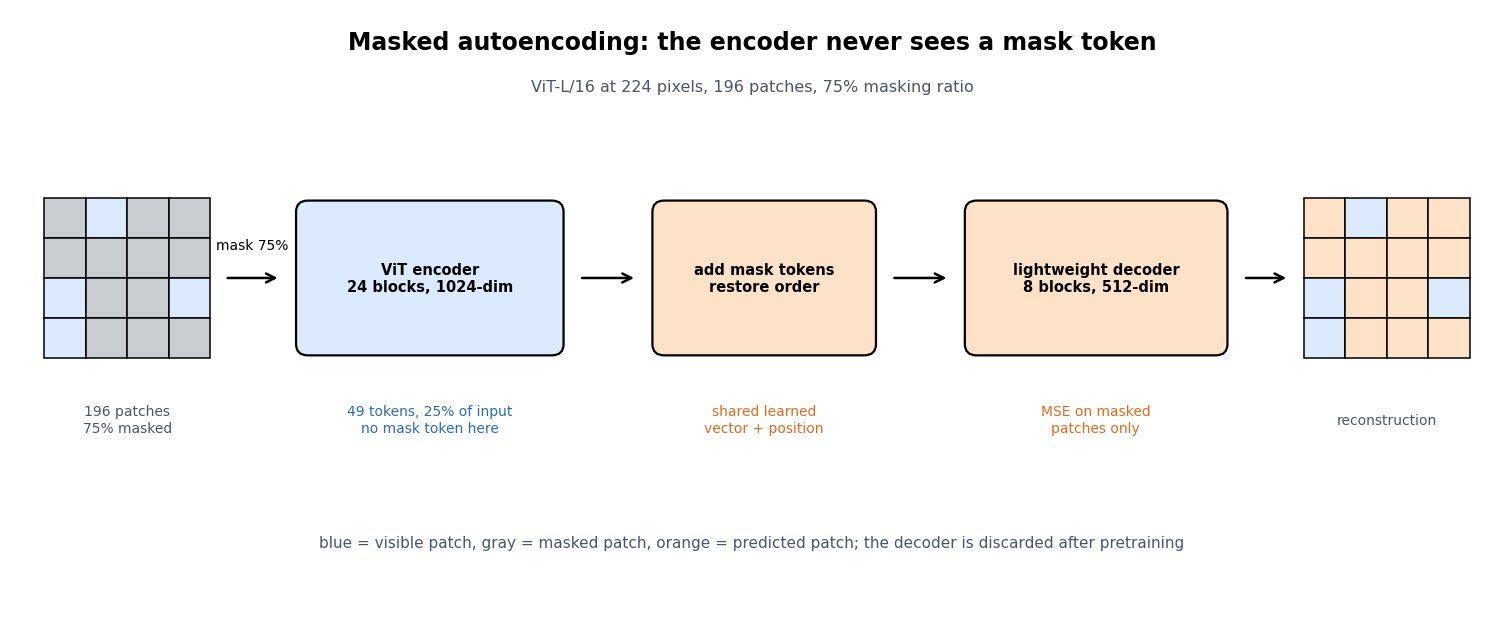
Flow diagram of the MAE pipeline: a 4 by 4 patch grid with 75 percent of cells masked, an arrow into a ViT encoder that processes only the 49 visible tokens, then a block that inserts mask tokens and restores order, then a lightweight 8-block decoder, then the reconstructed patch grid

Figure 1: The MAE pipeline for a ViT-L/16 at 224 pixels: of 196 patches only 49 reach the encoder, mask tokens are inserted just before a shallow decoder, and the MSE loss is computed on masked patches only.

Two details separate the text and vision instantiations. BERT cannot drop masked positions because the prediction head must sit at those positions, so the literal [MASK] symbol is fed to the encoder during pretraining and never appears at fine-tuning time; the original recipe patches this discrepancy by replacing only 80% of selected tokens with [MASK], 10% with a random token, and leaving 10% unchanged. MAE removes the problem structurally: masked patches are simply deleted from the encoder’s input sequence, and the mask token is a learned vector injected at the decoder. The second detail is the loss support. Computing the reconstruction error on masked patches only matters, since including visible patches lets the model spend capacity on an identity mapping and measurably hurts downstream accuracy.

Mathematical Formulation:
$\mathcal{L}_{\mathrm{MLM}} = -\sum_{i \in \mathcal{M}} \log p_{\theta}(x_i \mid \tilde{x})$
$\hat{x} = D\big(E(x_{\mathcal{V}}), m\big)$
$\mathcal{L}_{\mathrm{MAE}} = \frac{1}{|\mathcal{M}|} \sum_{i \in \mathcal{M}} \|\hat{x}_i - x_i\|_2^2$
$|\mathcal{V}| = (1 - \rho)\,N$
$C_{\mathrm{attn}}(\mathcal{V}) / C_{\mathrm{attn}}(N) = (1 - \rho)^2$

Where:

$\mathcal{L}_{\mathrm{MLM}}$ is the cross-entropy over masked token positions and $\mathcal{L}_{\mathrm{MAE}}$ the per-patch MSE; both are averaged over masked positions only.
$x_i$ is the true content at position $i$ , $\hat{x}_i$ the prediction, and $\tilde{x}$ the corrupted sequence containing $\texttt{[MASK]}$ symbols.
$\mathcal{M}$ and $\mathcal{V}$ are the masked and visible index sets, disjoint with $|\mathcal{M}| + |\mathcal{V}| = N$ for $N$ total tokens or patches.
$E$ is the deep encoder applied to visible tokens alone, $D$ the shallow decoder, and $m$ the shared learned mask-token embedding plus positional encoding.
$\rho$ is the masking ratio: $\rho = 0.15$ for BERT and $\rho = 0.75$ for MAE, giving $|\mathcal{V}| = 49$ of $N = 196$ patches.
$C_{\mathrm{attn}}$ is quadratic self-attention cost, so at $\rho = 0.75$ encoder attention drops to $1/16$ and the token-wise MLP cost to $1/4$ ; targets are usually per-patch normalized pixels rather than raw values.

Line chart of ImageNet top-1 accuracy against masking ratio from 10 to 90 percent, showing a nearly flat fine-tuning curve near 85 percent and a strongly peaked linear-probing curve rising to about 73.5 percent at a 75 percent masking ratio then falling sharply at 90 percent

Figure 2: Approximate ViT-L behaviour versus masking ratio: fine-tuning is nearly flat from 40% to 80%, while linear probing peaks sharply near 75%, which is why a ratio that looks extreme for text is the vision default.

Property	MAE (pixel targets)	MLM (BERT-style)	Contrastive / joint embedding
Corruption level	75% of patches removed	15% of tokens replaced or kept	No masking; two augmented views
Encoder input	Visible tokens only, no mask token	Full sequence including [MASK]	Full clean views
Prediction head	8-block 512-dim decoder, discarded	Single linear layer over the vocabulary	MLP projector plus temperature
Best transfer mode	Full fine-tuning and dense tasks	Fine-tuning on token-level tasks	Frozen features, k-NN, zero-shot retrieval
Main weakness	Capacity spent on high-frequency detail; weak linear probe	Only ~15% of positions produce gradient per step	Augmentation-sensitive; risk of collapse

August 16, 2026

DL0098 CLIP Zero-Shot Classification

What is CLIP, and how does contrastive image-text training enable zero-shot classification?

Answer

CLIP (Contrastive Language-Image Pre-training) is a dual-encoder model: an image encoder (a ViT or ResNet) and a text encoder (a Transformer) each map their input to a vector in one shared embedding space, and the vectors are L2-normalized so their inner product is a cosine similarity. Training uses a batch of $N$ image-caption pairs scraped from the web (400M pairs for the original model), computes the full $N \times N$ similarity matrix, and applies a symmetric InfoNCE loss that pushes the $N$ diagonal entries up and the $N^2 - N$ off-diagonal entries down. Nothing in that objective mentions class labels, so the learned text encoder is a general classifier generator: at test time you write each candidate class as a sentence such as “a photo of a golden retriever”, encode it, and the resulting unit vectors act as the rows of a linear classifier weight matrix. Classification is then one matrix multiply followed by an argmax over cosine similarities, which is why a new label set costs a text-encoder forward pass rather than a training run. The best original model (ViT-L/14@336px) reaches 76.2% zero-shot top-1 on ImageNet, matching a supervised ResNet-101 with an identical 76.2% ImageNet top-1 that saw 1.28M labeled images, and it is far more robust under distribution shift.

(1) Two Encoders, One Space: each modality has its own encoder plus a linear projection into a shared $d$ -dimensional space; there is no cross-attention between them, so image and text embeddings can be computed and cached independently.
(2) Symmetric InfoNCE Over The Batch: the loss is cross-entropy applied twice, once along rows (image picks its caption) and once along columns (caption picks its image), averaged.
(3) Learned Temperature: the logit scale $\exp(\tau)$ is a trained scalar initialized to a temperature of 0.07 and clipped at 100, which controls how hard the softmax pushes against near-miss negatives.
(4) Prompts Become Classifier Weights: zero-shot inference replaces the learned classification head with text embeddings of class descriptions, so the label set is defined at inference time, not at training time.
(5) Batch Size Is Part Of The Objective: negatives come only from the current batch, so the original model trained at $N = 32768$ across many GPUs with the similarity matrix sharded.

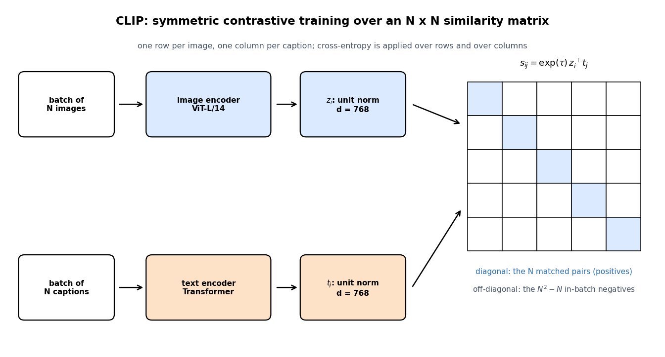
Diagram of CLIP training: a batch of N images passes through an image encoder to unit-norm vectors, a batch of N captions passes through a text encoder to unit-norm vectors, and both feed an N by N cosine similarity matrix whose diagonal cells are the positive pairs

Figure 1: Each training step builds the full $N \times N$ similarity matrix; the $N$ diagonal entries are the true pairs and every other entry is an in-batch negative, which is why one step at $N = 32768$ supplies over a billion contrastive comparisons.

Three details separate a working CLIP from a broken one. Normalization is load-bearing: without it the model can shrink the loss by inflating embedding norms instead of improving alignment, and the learned temperature then has no fixed scale to calibrate against. Prompt wording matters more than people expect, because captions in the training data are sentences, not bare nouns: using “a photo of a {label}” instead of the raw class name adds about 1.3 points on ImageNet, and ensembling 80 prompt templates by averaging their normalized text embeddings adds roughly 3.5 points for almost no inference cost, since the averaged vectors are computed once and cached. Finally, label naming is part of the model: polysemous class names such as “boxer” (dog breed or athlete) or “crane” (bird or machine) must be disambiguated in the prompt, which is a form of engineering that has no analogue in a supervised classifier with integer labels.

Mathematical Formulation:
$z_i = f_{\theta}(I_i) / \|f_{\theta}(I_i)\|_2$
$t_j = g_{\phi}(T_j) / \|g_{\phi}(T_j)\|_2$
$s_{ij} = \exp(\tau)\, z_i^{\top} t_j$
$\mathcal{L}_{I} = -\frac{1}{N}\sum_{i} \log \frac{e^{s_{ii}}}{\sum_{j} e^{s_{ij}}}$
$\mathcal{L} = \frac{1}{2}\left(\mathcal{L}_{I} + \mathcal{L}_{T}\right)$
$\hat{y} = \arg\max_{c} \; z^{\top} t_c$

Where:

$z_i$ and $t_j$ are the unit-norm embeddings of image $I_i$ and caption $T_j$ , both in $\mathbb{R}^{d}$ with $d = 768$ for ViT-L/14.
$f_{\theta}$ is the image encoder plus its projection and $g_{\phi}$ the text encoder plus its projection; the two share no weights.
$s_{ij}$ is the scaled cosine similarity and $\exp(\tau)$ the learned logit scale; since $z_i^{\top} t_j$ lies in $[-1, 1]$ , the scale alone sets the sharpness of the softmax.
$i, j \in \{1, \ldots, N\}$ index the batch; $\mathcal{L}_{I}$ normalizes each row and $\mathcal{L}_{T}$ the same expression with the softmax taken over columns.
$\hat{y}$ is the zero-shot prediction for a query image with embedding $z$ , and $t_c$ is the (optionally prompt-ensembled and renormalized) text embedding of class $c$ ; the temperature drops out of the argmax.
Required initial condition: $\tau = \log(1/0.07)$ at step 0, clamped so that $\exp(\tau) \leq 100$ throughout training to prevent the logits from exploding.

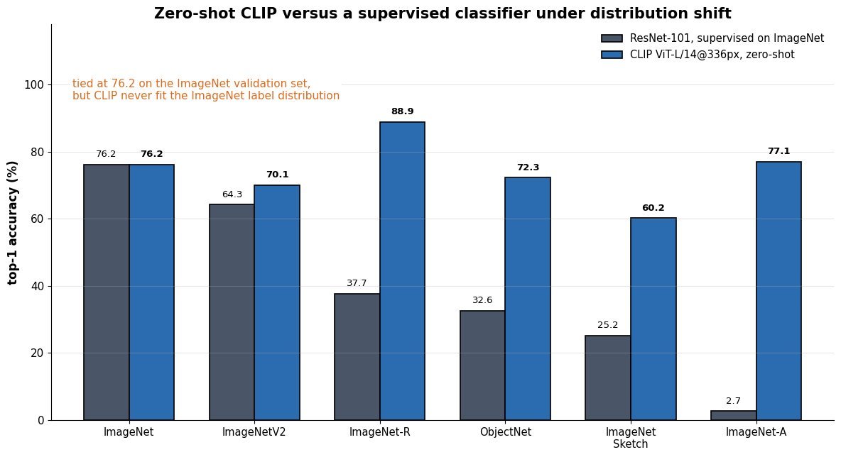
Grouped bar chart comparing top-1 accuracy of a supervised ResNet-101 and zero-shot CLIP ViT-L/14 on ImageNet and five distribution-shift benchmarks, with CLIP far ahead on ImageNet-R, ObjectNet, Sketch and ImageNet-A

Figure 2: Matched at 76.2% on the ImageNet validation set, the two models diverge sharply under shift: zero-shot CLIP keeps 77.1% on ImageNet-A and 60.2% on Sketch, where the supervised model drops to 2.7% and 25.2%, evidence that never fitting the ImageNet label distribution is itself a robustness mechanism.

Property	Zero-shot CLIP (ViT-L/14@336px)	Supervised classifier (ResNet-101)
Task supervision	Zero labeled examples for the task, 400M noisy web pairs for pretraining	1.28M hand-labeled images for exactly this label set
Adding a class	Encode one more prompt and append the vector, no gradient step	Collect labels, then retrain or refit the head
ImageNet top-1	76.2%	76.2%
ImageNet-A top-1	77.1%	2.7%
Specialized domains	Weak: near chance on tumor-patch classification, poor on counting and satellite land use	Strong once in-domain labels exist
Inference cost	One image forward pass plus a $d \times C$ matmul against cached text vectors	One forward pass through a fixed head

August 16, 2026

DL0097 Variational Autoencoder VAE

What is a variational autoencoder (VAE), and how does it differ from a plain autoencoder?

Answer

A variational autoencoder is a latent-variable generative model trained by amortized variational inference, not a compression network with a smaller bottleneck. A plain autoencoder learns a deterministic map $z = f_\phi(x)$ and minimizes reconstruction error alone, so nothing constrains where codes land: the latent space is an arbitrary point cloud with holes, and decoding a random vector usually produces garbage. A VAE instead makes the encoder output the parameters of a distribution $q_\phi(z|x) = \mathcal{N}(\mu_\phi(x), \sigma_\phi^2(x))$ , samples $z$ from it, and optimizes the evidence lower bound (ELBO), which adds a KL term pulling every posterior toward a fixed prior $p(z) = \mathcal{N}(0, I)$ . That single extra term is what turns an encoder-decoder pair into a generator: after training you can draw $z \sim \mathcal{N}(0, I)$ and decode it, because the aggregate posterior now covers the prior. The sampling step is made differentiable by the reparameterization trick, $z = \mu + \sigma \odot \epsilon$ with $\epsilon \sim \mathcal{N}(0, I)$ , which keeps the stochastic node out of the gradient path.

(1) Probabilistic Encoder: the encoder emits a mean and a log-variance per latent dimension rather than a point, so each input maps to a small blob of latent space instead of a single coordinate.
(2) Two-Term Objective: the loss is reconstruction plus a KL regularizer against the prior; a plain autoencoder has only the first term, which is exactly why it is not generative.
(3) Reparameterization Trick: sampling is rewritten as a deterministic function of the parameters and an external noise draw, giving a low-variance pathwise gradient instead of a high-variance score-function estimator.
(4) Sampling From The Prior: because the KL term forces the posteriors to overlap and fill the prior, ancestral sampling ( $z \sim p(z)$ , then decode) yields plausible data, and interpolation between two codes stays on the data manifold.
(5) Explicit Likelihood Bound: the ELBO is a lower bound on $\log p_\theta(x)$ , so a VAE gives a comparable density estimate, whereas an autoencoder’s reconstruction error has no probabilistic meaning.

Two-row diagram: the top row shows a plain autoencoder mapping input x through an encoder to a single deterministic code and back through a decoder; the bottom row shows a VAE whose encoder emits mu and log sigma squared, a sampling step z equals mu plus sigma times epsilon, and a decoder, with a KL term pulling the posterior toward the standard normal prior

Figure 1: The structural difference is one node: the plain autoencoder passes a single deterministic code to the decoder, while the VAE passes a sample from a learned Gaussian that the KL term keeps anchored to $\mathcal{N}(0, I)$ .

Two practical details dominate real training runs. The first is the balance between the two loss terms: with a strong decoder or a large KL weight, the cheapest solution is to set $q_\phi(z|x) = p(z)$ and ignore the latent entirely, a failure called posterior collapse that shows up as a KL term decaying to near zero while reconstruction stalls. Standard mitigations are KL annealing (ramp the weight from 0 to 1 over the first epochs) and free bits (do not penalize a dimension until its per-dimension KL exceeds a floor of roughly 0.05 to 0.5 nats). The second is the choice of likelihood: a diagonal Gaussian decoder is equivalent to an MSE reconstruction loss, which averages over plausible outputs and is the direct cause of the blurry samples VAEs are known for; discretized logistic or categorical likelihoods sharpen results noticeably. Modern image systems exploit this honestly, using a KL-regularized autoencoder as the perceptual compressor and putting the generative burden on a diffusion model in that latent space, as in Stable Diffusion.

Mathematical Formulation:
$\log p_\theta(x) \geq \mathcal{L}(\theta, \phi; x)$
$\mathcal{L} = \mathcal{L}_{rec} - \beta \, D_{KL}(q_\phi \| p)$
$\mathcal{L}_{rec} = \mathbb{E}_{q_\phi(z|x)}[\log p_\theta(x|z)]$
$q_\phi(z|x) = \mathcal{N}(\mu_\phi(x), \sigma_\phi^2(x))$
$z = \mu_\phi(x) + \sigma_\phi(x) \odot \epsilon$
$\epsilon \sim \mathcal{N}(0, I)$
$D_{KL} = -\frac{1}{2} \sum_{j=1}^{d} \delta_j$
$\delta_j = 1 + \log \sigma_j^2 - \mu_j^2 - \sigma_j^2$

Where:

$\mathcal{L}$ is the ELBO, a lower bound on the marginal log-likelihood $\log p_\theta(x)$ ; the gap between them equals $D_{KL}(q_\phi(z|x) \| p_\theta(z|x))$ , so maximizing the bound both fits the data and sharpens the approximate posterior.
$x$ is the observation and $z \in \mathbb{R}^{d}$ the latent code, with $d \ll \dim(x)$ in the usual bottleneck setting.
$q_\phi(z|x)$ is the encoder (recognition model) with parameters $\phi$ , and $p_\theta(x|z)$ is the decoder (likelihood) with parameters $\theta$ .
$p(z) = \mathcal{N}(0, I)$ is the fixed prior, and $j \in \{1, \ldots, d\}$ indexes latent dimensions in the closed-form KL, where $\mu_j$ and $\sigma_j$ are the encoder outputs for example $x$ .
$\odot$ is elementwise multiplication and $\epsilon$ is the external noise draw that makes the sample differentiable in $\mu$ and $\sigma$ .
$\beta$ is the KL weight; $\beta = 1$ recovers the exact ELBO, $\beta > 1$ gives the beta-VAE disentanglement regime, and $\beta = 0$ degenerates to a plain autoencoder. Networks are typically initialized so $\log \sigma_j^2 \approx 0$ , which starts training near the prior.

Two scatter panels of a two-dimensional latent space: on the left the plain autoencoder codes sit in six distant clusters far from the origin with large empty gaps and prior samples falling in a hole, on the right the VAE codes form overlapping blobs filling the unit and two-sigma circles of the standard normal prior so prior samples land on data

Figure 2: Encoded training data in a 2D latent space. The plain autoencoder is free to scatter codes anywhere, so a draw from $\mathcal{N}(0, I)$ lands in a hole; the KL term compresses the VAE’s aggregate posterior onto the prior, so the same draw hits populated territory.

Property	Plain Autoencoder	VAE	VQ-VAE
Encoder output	One deterministic code vector per input	Distribution parameters, mean and log-variance	Continuous vector snapped to the nearest codebook entry
Training objective	Reconstruction error only	ELBO: reconstruction minus beta times KL to N(0, I)	Reconstruction plus codebook and commitment losses, no KL
Latent geometry	Arbitrary scale, holes and gaps between clusters	Smooth and prior-matched, interpolation stays on-manifold	Discrete grid of K entries, no notion of interpolation
Generating new data	Not supported, a random code decodes to noise	Draw z from the prior and decode, one forward pass	Needs a learned prior over codes, such as a transformer
Typical failure	Memorizes an identity map when the bottleneck is wide	Posterior collapse, blurry Gaussian-likelihood samples	Codebook collapse with most entries unused
Common use	Denoising, compression, anomaly detection	Generative modeling and the latent space of latent diffusion	Discrete tokens for autoregressive image and audio models

August 16, 2026

DL0096 Autoencoders Practical Uses

What is an autoencoder? What are the practical uses of autoencoders?

Answer

An autoencoder is a network trained to reconstruct its own input through a narrow bottleneck: an encoder maps $x \in \mathbb{R}^{D}$ to a code $z \in \mathbb{R}^{d}$ with $d \ll D$ , and a decoder maps that code back to $\hat{x}$ , with the reconstruction error as the only supervision. Because the target is the input itself, training needs no labels, which is why autoencoders are the canonical self-supervised compression model. The bottleneck is what makes the code useful: the network cannot pass everything through, so it must keep the structure that is shared across typical inputs and drop the rest. With linear encoder and decoder and squared loss, the optimum spans exactly the same subspace as the top $d$ principal components; nonlinear layers buy a curved manifold instead of a flat one. The practical uses split into three families depending on which part of the trained model you keep: the error (anomaly detection), the code (compression, retrieval, visualization, latent space for a diffusion model), or the decoder (denoising, inpainting, generation once the latent is regularized).

(1) Bottleneck Plus Reconstruction Loss: the objective is $\|x - \hat{x}\|_2^2$ (or cross-entropy for binary pixels), and the capacity constraint, not the loss, is what forces a compressed representation.
(2) Undercomplete Versus Regularized: an undercomplete model constrains $d$ directly, while sparse, denoising, and contractive variants keep a wide code and constrain it with an $L_1$ penalty, input corruption, or a Jacobian penalty.
(3) Linear Case Recovers PCA: a single linear layer each side with MSE learns the principal subspace, so any gain over PCA must come from nonlinearity, not from the architecture being a neural network.
(4) Anomaly Detection By Error Score: train only on normal data, then score new samples with $s(x) = \|x - \hat{x}\|_2^2$ and flag $s(x) > \tau$ , with $\tau$ set from a percentile of validation errors.
(5) Compression Into A Working Latent Space: modern latent diffusion models run denoising inside an autoencoder latent that shrinks a $512 \times 512 \times 3$ image to $64 \times 64 \times 4$ , a 48x reduction in elements, which is what makes high-resolution sampling affordable.
(6) Not Generative By Default: a vanilla autoencoder learns no density over $z$ , so decoding an arbitrary code usually yields garbage; sampling requires a VAE, VQ-VAE, or a prior fitted over the codes afterwards.

Diagram of an autoencoder: a 784-dimensional input passes through a 256-unit hidden layer into a 32-dimensional code, then back out through a 256-unit hidden layer to a 784-dimensional reconstruction, with both ends feeding a reconstruction loss box

Figure 1: The flow is $x$ → $z$ → $\hat{x}$ ; the $784 \rightarrow 32$ bottleneck is a 24.5x squeeze, and nothing but the reconstruction error supervises what the code contains.

Where do they actually earn their place in a system? Anomaly detection on sensor, telemetry, and transaction data is the most common production use, because normal data is abundant and labeled failures are not. Denoising and restoration use the decoder: train with corrupted inputs and clean targets, and the model learns to project back onto the data manifold. Dimensionality reduction gives a cheap nonlinear preprocessor, typically compressing to 32 or 64 dimensions before a nearest-neighbor index or a t-SNE plot, which is far cheaper than running the visualization on raw features. Two uses dominate current deep learning: the perceptual autoencoder that provides the latent space for latent diffusion, and masked autoencoders, where a ViT reconstructs 75% masked patches as a pretraining task and the encoder is then fine-tuned for classification or detection. Recommender systems also use the pattern directly, reconstructing a user’s sparse interaction vector to predict the entries that are missing.

Histogram of reconstruction errors: normal samples cluster at low error, anomalous samples spread into a long right tail, with a vertical threshold line drawn at the 99th percentile of the normal validation errors

Figure 2: Illustrative anomaly scores from an autoencoder trained on normal data only. A threshold at the 99th percentile of normal validation errors fixes the false-positive rate at 1% by construction, and the achievable recall depends entirely on how far the anomalous tail separates.

Mathematical Formulation:
$z = f_{\theta}(x)$
$\hat{x} = g_{\phi}(z)$
$\mathcal{L}(\theta, \phi) = \frac{1}{N} \sum_{i=1}^{N} \| x_i - \hat{x}_i \|_2^2$
$s(x) = \| x - g_{\phi}(f_{\theta}(x)) \|_2^2$
$\mathcal{L}_{\mathrm{DAE}} = \mathbb{E} \| x - g_{\phi}(f_{\theta}(\tilde{x})) \|_2^2$

Where:

$z \in \mathbb{R}^{d}$ is the code and $\hat{x} \in \mathbb{R}^{D}$ the reconstruction of the input $x \in \mathbb{R}^{D}$ .
$D$ is the input dimension and $d$ the code dimension, with $d \ll D$ in the undercomplete case.
$f_{\theta}$ is the encoder and $g_{\phi}$ the decoder, with trainable parameters $\theta$ and $\phi$ optimized jointly.
$i \in \{1, \ldots, N\}$ indexes the $N$ training examples, and $\mathcal{L}$ is the mean squared reconstruction loss.
$s(x)$ is the anomaly score, and a sample is flagged when $s(x) > \tau$ for a threshold $\tau$ chosen from a high percentile of normal validation scores.
$\tilde{x}$ is a corrupted copy of $x$ (additive noise, masking, or dropout on inputs); the denoising objective still targets the clean $x$ , which is what prevents the identity solution even when $d \geq D$ .

Property	Undercomplete autoencoder	PCA	VAE
Mapping	Nonlinear encoder and decoder, learned by SGD	Single linear projection, closed-form via SVD	Nonlinear, but the encoder outputs a distribution over z
Objective	Reconstruction error only	Maximum retained variance, equivalent to linear MSE	Reconstruction plus a KL term pulling z toward a prior
Latent geometry	Arbitrary, often with holes and unused directions	Orthogonal ordered axes, fully interpretable scale	Smooth and roughly isotropic, so interpolation is meaningful
Sampling new data	Not supported without fitting a prior over codes afterwards	Only under an explicit Gaussian model such as probabilistic PCA	Yes, sample the prior and decode
Typical use	Anomaly scoring, denoising, compact features for indexing	Fast baseline, whitening, exploratory analysis	Latent space for diffusion, generative sampling, recsys
Main caveat	Too much capacity collapses to near-identity and the code stops being informative	Cannot represent curved manifolds; cost grows with feature count	Blurry reconstructions and posterior collapse if the KL weight is too high

August 16, 2026

ML0005 Discriminative and Generative
What are the differences between discriminative and generative models?
Answer
Discriminative models learn to draw a boundary between classes: they model the conditional probability $P(y \mid x)$ directly, mapping features $x$ to labels $y$ without modeling how the data was generated. Examples include logistic regression, support vector machines, and neural network classifiers. Generative models instead estimate the joint probability $P(x, y)$ (via $P(x \mid y)$ and $P(y)$ ), capturing how the data itself is generated, and then use Bayes’ theorem to derive $P(y \mid x)$ for classification. Examples include Naive Bayes, hidden Markov models, VAEs, and GANs. Because generative models learn the data distribution, they can also sample new data; discriminative models can only separate existing classes.
(1) Modeling Target: Discriminative models learn $P(y \mid x)$ directly; generative models learn $P(x, y)$ or $P(x \mid y) P(y)$ .
(2) Decision Mechanism: Discriminative models find a decision boundary; generative models compare class-conditional densities through Bayes’ rule.
(3) Capabilities: Discriminative models only classify; generative models can also generate samples, handle missing features, and score outliers.

Figure 1: Left: a discriminative model cares only about the boundary between classes. Right: a generative model fits a distribution to each class, capturing how the data itself looks.
Mathematical Formulation:
$\text{discriminative:} \quad \hat{y} = \arg\max_y \, P(y \mid x)$
$\text{generative:} \quad P(y \mid x) = \frac{P(x \mid y)\, P(y)}{P(x)}$
Where:
$\hat{y}$ is the predicted label and $y$ ranges over the class set for input $x$ .
$P(y \mid x)$ is the posterior, the quantity a discriminative model learns directly.
$P(x \mid y)$ is the class-conditional likelihood (how data of class $y$ looks) and $P(y)$ the class prior; together they define the joint $P(x, y)$ a generative model learns.
$P(x)$ is the evidence normalizer, computable as $\sum_y P(x \mid y) P(y)$ over all classes.
Login to view more content
February 26, 2025

Tag: GenAI

DL0099 Masked Autoencoding MAE

DL0098 CLIP Zero-Shot Classification

DL0097 Variational Autoencoder VAE

DL0096 Autoencoders Practical Uses

ML0005 Discriminative and Generative