Interview for Machine Learning

Tag: Loss

DL0047 Focal Loss II
Please compare focal loss and weighted cross-entropy.
Answer
Weighted Cross-Entropy (WCE) rescales loss by class to correct prior imbalance and is simple and robust for noisy labels; Focal Loss (FL) multiplies cross-entropy by a difficulty-dependent factor $\gamma$ to suppress easy-example gradients and focus learning on hard examples, making it preferable when many easy negatives overwhelm training but requiring careful tuning to avoid amplifying label noise.
$\text{WeightedCE}(p_t) = -\alpha_t \log(p_t)$
Where:
$p_t$ is the model probability for the ground-truth class;
$\alpha_t$ is the per-class weight for class t.
$\text{FocalLoss}(p_t) = -\alpha_t (1 - p_t)^\gamma \log(p_t)$
Where:
$p_t$ is the model probability for the ground-truth class;
$\alpha_t$ is the optional per-class weight for class t;
$\gamma \ge 0$ is the focusing parameter that down-weights easy examples.
Here is a table to compare focal loss and weighted cross-entropy.
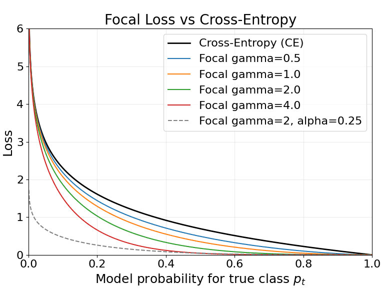
The figure below compares Cross-Entropy, Weighted Cross-Entropy, and Focal Loss.
Login to view more content
October 27, 2025
DL0046 Focal Loss
What is focal loss, and why does it help with class imbalance?
Answer
Focal loss augments cross-entropy with a modulating term $(1 - p_t)^\gamma$ and an optional balancing weight $\alpha_t$ to suppress gradients from easy, majority-class examples and amplify learning from hard or minority-class examples, improving performance in severe class-imbalance settings when hyperparameters are properly tuned.
(1) Focal loss formula:
$\text{FocalLoss}(p_t) = -\alpha_t (1 - p_t)^\gamma \log(p_t)$
Where:
$p_t$ is the model probability for the ground-truth class;
$\gamma \ge 0$ is the focusing parameter that down-weights easy examples;
$\alpha_t \in (0,1)$ is an optional class-balancing weight for class t.
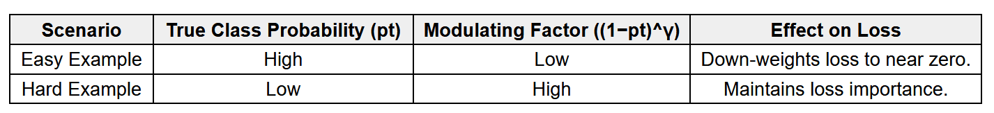
(2) Modulation: The factor $(1 - p_t)^\gamma$ reduces loss from well-classified (high-confidence) examples, concentrating gradients on hard / low-confidence examples.

(3) Class imbalance effect:
In cross-entropy, abundant, easy negatives still produce a large total gradient, dominating learning.
Focal loss down-weights those contributions, ensuring rare/difficult samples have a stronger influence.
The plot below shows cross-entropy and focal-loss curves for several $\gamma$ values and an example $\alpha$ .
Login to view more content
October 27, 2025
ML0053 Hinge Loss for SVM
Explain the Hinge Loss function used in SVM.
Answer
The Hinge Loss function is a key element in Support Vector Machines that penalizes both misclassified points and correctly classified points that lie within the decision margin. It assigns zero loss to points that are correctly classified and lie outside or exactly on the margin, and applies a linearly increasing loss as points move closer to or across the decision boundary. This loss structure encourages the SVM to maximize the margin between classes, promoting robust and generalizable decision boundaries.
The Hinge Loss is defined as follows.
$\text{Hinge Loss} = \max(0,\ 1 - y \cdot f(\mathbf{x}))$
Where:
$y \in {-1, +1}$ is the true label,
$f(\mathbf{x})$ is the raw model output.
Hinge Loss is plotted in the figure below.
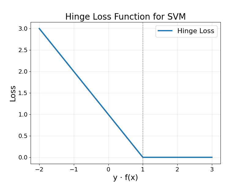
Zero Loss: When $y \cdot f(\mathbf{x}) \ge 1$ , meaning the point is correctly classified with margin.
Positive Loss: When $y \cdot f(\mathbf{x}) < 1$ , the point is either inside the margin or misclassified.
Login to view more content
June 11, 2025
ML0050 Logistic Regression III
Why is Mean Squared Error (L2 Loss) an unsuitable loss function for logistic regression compared to cross-entropy?
Answer
Mean Squared Error (MSE) is unsuitable for logistic regression primarily because, when combined with the sigmoid function, it can lead to a non-convex loss landscape, making optimization harder and increasing the risk of poor convergence. Additionally, it provides weaker gradients when predictions are confidently incorrect, slowing down learning. Cross-entropy loss is better suited as it aligns with the Bernoulli distribution assumption, produces stronger gradients, and leads to a well-behaved convex loss for a single neuron binary classification setting.
(1) Wrong Assumption: MSE assumes a Gaussian distribution of errors, while logistic regression assumes a Bernoulli (binary) distribution.
(2) Non-convex Optimization: MSE with sigmoid can create a non-convex loss surface, making optimization harder and less stable.
(3) Gradient Issues: MSE leads to smaller gradients for confident wrong predictions, slowing down learning compared to cross-entropy.
(4) Interpretation: Cross-entropy directly compares predicted probabilities to true labels, which is more appropriate for classification.
The figure below shows the non-convex loss surface when MSE is used for logistic regression.
Login to view more content
June 10, 2025
ML0022 Cross Entropy Loss
Explain how Cross Entropy Loss is used for a classification task.
Answer
Cross-entropy loss, also known as log loss or logistic loss, is a commonly used loss function in machine learning, particularly for classification tasks. It quantifies the difference between two probability distributions: the predicted probabilities generated by a model and the true probability distribution of the target variable. The goal of training a classification model is to minimize this loss.
For binary classification:
${\large \text{Binary Cross-Entropy Loss} = - \displaystyle\frac{1}{n}\sum_{i=1}^{n} [y_i \cdot \log(p_i) + (1-y_i) \cdot \log(1-p_i)]}$
where:
${\large n}$ is the number of total samples.
${\large y_i}$ is the true label (0 or 1) for the i-th data point.
${\large p_i}$ is the predicted probability of the positive class (class 1) for the i-th data point.
For multi-class classification:
${\large \text{Categorical Cross-Entropy Loss} = - \displaystyle\frac{1}{n}\sum_{i=1}^{n} \sum_{j=1}^{C} y_{ij} \cdot \log(p_{ij})}$
where:
${\large n}$ is the number of total samples.
${\large C}$ is the number of classes.
${\large y_{ij}}$ is a binary indicator (0 or 1) that is 1 if the true class for the i-th data point is j, and 0 otherwise (one-hot encoding).
${\large p_{ij}}$ is the predicted probability that the i-th data point belongs to class j.
The logarithm function in the formula penalizes incorrect predictions more severely when the model is more confident about that incorrect prediction.
For a true label of 1, the loss is higher when the predicted probability p is closer to 0, and lower when p is closer to 1.
For a true label of 0, the loss is higher when the predicted probability p is closer to 1, and lower when p is closer to 0.
The cross-entropy loss approaches 0 when the predicted probability distribution is close to the true distribution.
Key Properties:
Differentiable: The cross-entropy loss function is differentiable, which is essential for gradient-based optimization algorithms.
Sensitive to Confidence: It strongly penalizes confident but incorrect predictions.
Probabilistic Interpretation: It directly works with the predicted probabilities of the classes.
Login to view more content
March 31, 2025
ML0021 L1 Loss L2 Loss
What are the key differences between L1 loss and L2 loss?
Answer
L1 Loss (Mean Absolute Error – MAE)
L1 loss measures the average absolute difference between the actual and predicted values. It is expressed as:
${\large \text{L1 Loss} = \displaystyle\frac{1}{n}\sum_{i=1}^{n} | \hat{y}_i - y_i |}$
Where,
${\large y_i}$ represents the actual value for the i-th data point.
${\large\hat{y}_i}$ represents the predicted value for the i-th data point.
${\large n}$ is the total number of data points.
Sensitivity to Outliers: L1 loss is less sensitive to outliers because it treats all errors equally. A large error has a proportional impact on the total loss.
Gradient Behavior: The gradient of the L1 loss is constant (+1 or -1) for non-zero errors. At zero error, the gradient is undefined. This can lead to instability during optimization near the optimal solution.
Sparsity: L1 loss has a tendency to produce sparse models, meaning it can drive the weights of less important features to exactly zero. This is a desirable property for feature selection.
L2 Loss (Mean Squared Error – MSE)
L2 loss measures the average squared difference between the actual and predicted values. It is expressed as:
${\large \text{L2 Loss} = \displaystyle\frac{1}{n}\sum_{i=1}^{n} (\hat{y}_i - y_i)^2}$
Where,
${\large y_i}$ represents the actual value for the i-th data point.
${\large\hat{y}_i}$ represents the predicted value for the i-th data point.
${\large n}$ is the total number of data points.
Sensitivity to Outliers: L2 loss is more sensitive to outliers because it squares the errors. A large error has a disproportionately larger impact on the total loss, making the model more influenced by extreme values.
Gradient Behavior: The gradient of the L2 loss is proportional to the error (2( ${\large y_i}$ – ${\large\hat{y}_i}$ )). This means that larger errors have larger gradients, which can help the optimization process converge faster when the errors are large. As the error approaches zero, the gradient also approaches zero, leading to more stable convergence near the optimal solution.
Sparsity: L2 loss does not inherently lead to sparse models. It tends to shrink the weights of all features, but rarely drives them to exactly zero.
Login to view more content
March 29, 2025
ML0001 Loss Curve Plot
The following training loss curves were plotted with different experiment settings. Which of these training loss curves most likely indicates the correct experiment settings?
Answer
A
Explanation:
In an ideal training environment, the training loss is expected to diminish steadily over time. This indicates that the model is learning and improving its performance over time.
Login to view more content
February 23, 2025