ML0053 Hinge Loss for SVM

The Hinge Loss function is a key element in Support Vector Machines that penalizes both misclassified points and correctly classified points that lie within the decision margin. It assigns zero loss to points that are correctly classified and lie outside or exactly on the margin, and applies a linearly increasing loss as points move closer to or across the decision boundary. This loss structure encourages the SVM to maximize the margin between classes, promoting robust and generalizable decision boundaries.

The Hinge Loss is defined as follows.

Where:
is the true label,
is the raw model output.

Hinge Loss is plotted in the figure below.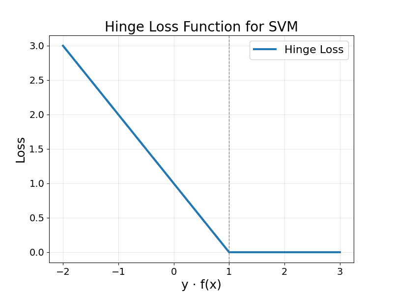

Zero Loss: When , meaning the point is correctly classified with margin.
Positive Loss: When , the point is either inside the margin or misclassified.