Tag: Stats

ML0096 Maximum Likelihood Estimation

What is maximum likelihood estimation (MLE), and how does it connect to the cross-entropy loss used in modern neural network training?

Answer

Maximum likelihood estimation is a method for estimating the parameters of a statistical model by finding the parameter values that make the observed data most probable. Given a dataset and a parametric model, MLE chooses the parameters that maximize the likelihood function: the joint probability of the observed data under the model. Equivalently, we maximize the log-likelihood, which converts the product of probabilities into a sum of log-probabilities, making optimization tractable and numerically stable. MLE is the foundation of most modern ML training: an ICLR 2025 blog post explicitly derives the standard classification cross-entropy loss from the MLE principle, showing that minimizing cross-entropy is equivalent to maximizing the conditional log-likelihood of the training data under the model. For a simple coin flip example, if you observe 3 heads in 4 flips, the MLE of the heads probability is simply 3/4, the sample proportion.

(1) Likelihood vs Probability: probability is the chance of data given fixed parameters; likelihood is the same function viewed as a function of parameters with the data fixed, and MLE finds the parameters that maximize it.
(2) Log-Likelihood Trick: taking the log converts the product $\prod P(x_i \mid \theta)$ into the sum $\sum \log P(x_i \mid \theta)$ , which is easier to differentiate, numerically stable, and decomposes additively over data points for stochastic gradient descent.
(3) Connection to Production ML: an ICLR 2025 blog derives cross-entropy loss as the negative log-likelihood under a categorical model, so training a classifier with cross-entropy is MLE; logistic regression is MLE under a Bernoulli model, and linear regression with squared error is MLE under a Gaussian noise model.

Top panel: the likelihood curve L(theta) = theta^3 (1-theta) over theta from 0 to 1, peaking at theta = 0.75 where a dashed line and diamond marker label the MLE; bottom panel: the log-likelihood 3 ln(theta) + ln(1-theta), peaking at the same 0.75

Figure 1: Coin flip MLE: with 3 heads in 4 flips, the likelihood $L(\theta) = \theta^3(1-\theta)$ and log-likelihood $3\ln\theta + \ln(1-\theta)$ both peak at $\hat{\theta} = 3/4 = 0.75$ , the sample proportion of heads.

The coin flip example makes the principle concrete. Suppose you flip a coin 4 times and observe 3 heads and 1 tail. The coin has an unknown probability $\theta$ of heads. The likelihood of observing this data is $L(\theta) = \theta^3 (1 - \theta)^1$ , and the log-likelihood is $\ell(\theta) = 3 \ln \theta + \ln(1 - \theta)$ . Taking the derivative and setting it to zero gives $3/\theta - 1/(1-\theta) = 0$ , which solves to $\hat{\theta} = 3/4$ . This is the sample proportion, and it is the MLE because the likelihood is maximized there. The same principle scales to neural networks: the cross-entropy loss $L = -\frac{1}{N}\sum_i \log q_\theta(y_i \mid x_i)$ is the negative average log-likelihood, and gradient descent on this loss is MLE for the network’s parameters. A 2024 arXiv paper established finite-sample guarantees for MLE in logistic regression, showing the sample complexity depends on both dimension and signal strength, with distinct regimes at different signal-to-noise ratios.

Mathematical Formulation:
$\hat{\theta}_{\mathrm{MLE}} = \arg\max_{\theta}\; \prod_{i=1}^{N} P(x_i \mid \theta)$
$\ell(\theta) = \sum_{i=1}^{N} \log P(x_i \mid \theta)$
$\hat{\theta}_{\mathrm{MLE}} = \arg\max_{\theta}\; \ell(\theta)$

Where:

$\hat{\theta}_{\mathrm{MLE}}$ is the parameter value that maximizes the likelihood; $P(x_i \mid \theta)$ is the probability of observation $x_i$ under the model with parameters $\theta$ .
$\ell(\theta)$ is the log-likelihood, which converts the product into a sum for tractability; maximizing $\ell$ is equivalent to maximizing the likelihood because log is monotonically increasing.
For the coin flip: $\ell(\theta) = N_H \ln \theta + N_T \ln(1 - \theta)$ , and setting $d\ell/d\theta = 0$ gives $\hat{\theta} = N_H / (N_H + N_T)$ , the sample proportion. For classification: $\ell = \sum_i \log q_\theta(y_i \mid x_i)$ , and minimizing $-\ell/N$ is the cross-entropy loss.

Model	Likelihood	MLE Solution	Equivalent Loss
Bernoulli (coin)	theta^NH (1-theta)^NT	NH / (NH + NT)	Binary cross-entropy
Gaussian (regression)	prod N(yi \| f(xi), sigma^2)	Least squares solution	Mean squared error
Categorical (classifier)	prod q_theta(yi \| xi)	Gradient descent on -log q	Cross-entropy loss

August 12, 2026

ML0095 Confidence Interval

What is a confidence interval, and what is the correct interpretation of a 95% confidence interval, as used in sequential A/B testing and experimentation platforms?

Answer

A confidence interval is a range computed from sample data that is designed to contain an unknown population parameter with a specified probability under repeated sampling. The correct frequentist interpretation of a 95% confidence interval is: if you repeated the experiment many times, computing a new interval from each sample, about 95% of those intervals would contain the true parameter. It is a statement about the procedure, not about any single interval. Once data is observed, the true parameter is either inside your specific interval or not (probability 0 or 1); you cannot say “there is a 95% probability the parameter is in this interval,” because that is a Bayesian credible interval interpretation requiring a prior. Sequential A/B testing platforms use “anytime-valid” confidence sequences that maintain this coverage guarantee across continuous monitoring, and asymmetric experiment designs treat confidence interval width as a design parameter controlled through sample allocation between test and control groups.

(1) Procedure vs Single Interval: the 95% refers to the long-run coverage rate of the interval-construction procedure across hypothetical repeated samples, not the probability that the true parameter is in any one observed interval.
(2) Frequentist vs Bayesian: saying “95% probability the parameter is in this interval” is a Bayesian credible interval statement; a 2024 paper showed this distinction has real business impact, as frequentist estimators overstate A/B test effect sizes (winner’s curse) while Bayesian estimators with correct priors do not.
(3) Production Use: anytime-valid confidence sequences enable canary testing so the 95% coverage holds throughout continuous monitoring, not just at a pre-specified endpoint; asymmetric experiment designs optimize CI width by nonlinearly increasing control group size when shrinking test group size (40% test reduction requires 3x control increase).

Twenty horizontal confidence intervals computed from repeated samples, with a vertical line at the true parameter value; about 19 of 20 intervals cross the true value while one misses it, illustrating 95% coverage

Figure 1: The frequentist interpretation: across 20 repeated experiments, about 19 of the 95% confidence intervals contain the true parameter (vertical line); the 95% is a property of the procedure, not of any single interval.

The width of a confidence interval depends on three things: the confidence level (higher confidence means wider intervals), the sample size (larger n means narrower intervals), and the variability of the data (higher variance means wider intervals). For a mean with known variance, the 95% CI is the sample mean plus or minus 1.96 standard errors. When the variance is unknown and estimated from the sample, the t-distribution replaces the normal, giving slightly wider intervals for small samples. A critical production issue is peeking: repeatedly checking whether a confidence interval excludes zero and stopping when it does inflates the false positive rate, because each check is a separate test. Anytime-valid confidence sequences solve this by using a test statistic whose coverage guarantee holds uniformly over time, so you can monitor continuously without breaking the 95% promise. Conformal prediction (2024-2025) extends the idea to distribution-free prediction intervals for ML models, providing finite-sample coverage without normality assumptions.

Mathematical Formulation:
$\bar{x} \pm z_{\alpha/2}\, \frac{\sigma}{\sqrt{n}}$
$P\!\left(\bar{X} - z_{\alpha/2}\frac{\sigma}{\sqrt{n}} \leq \mu \leq \bar{X} + z_{\alpha/2}\frac{\sigma}{\sqrt{n}}\right) = 1 - \alpha$

Where:

$\bar{x}$ is the sample mean, $\sigma$ is the population standard deviation (replaced by sample standard deviation $s$ with the t-distribution when unknown), and $n$ is the sample size.
$z_{\alpha/2}$ is the critical value of the standard normal at level $\alpha/2$ ; for 95% confidence, $\alpha = 0.05$ and $z_{0.025} = 1.96$ .
The probability statement is over the random interval (which depends on $\bar{X}$ ), not over the fixed parameter $\mu$ ; this is the frequentist distinction. The interval either covers $\mu$ or not for any single sample, but the procedure covers it $1 - \alpha$ of the time across repeated samples.

Concept	Frequentist CI	Bayesian Credible Interval
Interpretation	95% of repeated-sample intervals contain the true value	95% probability the parameter is in this interval
Requires Prior?	No	Yes (prior over the parameter)
Parameter Is	Fixed, unknown constant	Random variable with a distribution
Production Note	Frequentist: winner’s curse overstates effect sizes	Bayesian: correct priors avoid winner’s curse

August 12, 2026

ML0092 Naive Bayes for Continuous Features

How does Naive Bayes handle continuous numeric features, and what goes wrong when the Gaussian assumption is violated?

Answer

The default approach is Gaussian Naive Bayes: for each continuous feature, the model estimates a per-class mean and variance from the training data and plugs the feature value into the Gaussian PDF to get the likelihood. This is fast (one pass to compute mean and variance, O(nd)) and works well when features are approximately normal within each class, as in the Iris dataset or standardized medical lab values. The problem is that the Gaussian assumption is often violated: income is right-skewed, reaction times are log-normal, and sensor readings can be multi-modal. When the true distribution is skewed or has heavy tails, the Gaussian likelihood misestimates the probability mass, pushing the posterior toward 0 or 1 incorrectly. The fixes are discretization (bin the feature and use Categorical or Multinomial NB), kernel density estimation (replace the parametric Gaussian with a non-parametric KDE), or transformation (log or Box-Cox transform to normalize the feature before applying Gaussian NB).

(1) Gaussian NB (Default): estimates $\mu_{yj}$ and $\sigma_{yj}^2$ per class per feature, then uses the Gaussian PDF in the likelihood product; O(nd) training, O(d) prediction, but assumes normality.
(2) Discretization: bin the continuous feature into k bins (equal-width or quantile), then treat it as categorical with k values; the 2024 Max-Relevance-Min-Divergence (MRmD) method beats prior discretization schemes on most of 45 benchmark datasets by maximizing discriminant information and generalization simultaneously.
(3) Kernel Density Estimation: replace the Gaussian with a non-parametric KDE $\hat{f}(x \mid y) = \frac{1}{n_y h}\sum K(\frac{x - x_i}{h})$ ; the R naivebayes package and MATLAB’s ClassificationNaiveBayes both support it, and a 2025 paper used optimized robust KDE with Welsch M-estimation to handle outliers in Bayesian classification.

Three panels: left shows a skewed income distribution with a Gaussian fit that misses the long tail; middle shows discretization into bins with per-class bin probabilities; right shows a KDE curve that follows the true skewed shape closely

Figure 1: Three approaches to continuous features in Naive Bayes: Gaussian NB fits a normal curve that misses skewness, discretization bins the feature into categorical probabilities, and kernel density estimation follows the true non-parametric shape.

The practical decision flow is: start with Gaussian NB and check the per-class histograms. If the feature is approximately normal within each class, Gaussian is fine and is the cheapest option. If the feature is skewed but unimodal, apply a log or Box-Cox transform and re-check normality. If the feature is multi-modal or has heavy tails that resist transformation, use discretization (simpler, faster, but loses information) or KDE (more accurate, but slower at prediction because it evaluates the kernel against all training points in that class). Scikit-learn’s GaussianNB also tends to produce overconfident probabilities because the independence assumption compounds with the Gaussian misfit, so CalibratedClassifierCV with isotonic regression is recommended when the predicted probabilities need to be reliable, as in a medical risk score where the probability itself (not just the classification) drives the decision.

Mathematical Formulation:
$P(x_j \mid y) = \frac{1}{\sqrt{2\pi\sigma_{yj}^2}} \exp\!\left(-\frac{(x_j - \mu_{yj})^2}{2\sigma_{yj}^2}\right)$
$\hat{f}_h(x \mid y) = \frac{1}{n_y h} \sum_{i=1}^{n_y} K\!\left(\frac{x - x_i^{(y)}}{h}\right)$

Where:

The first equation is Gaussian NB: $\mu_{yj}$ and $\sigma_{yj}^2$ are the class-conditional mean and variance of feature $j$ , estimated as the sample mean and variance of all training values of feature $j$ in class $y$ .
The second equation is kernel density estimation: $n_y$ is the number of training points in class $y$ , $h$ is the bandwidth, $K$ is the kernel function (typically Gaussian), and $x_i^{(y)}$ are the training values of the feature in class $y$ .
For discretization, the continuous range is split into $k$ bins, and $P(\text{bin}_b \mid y) = (N_{yb} + \alpha) / (N_y + \alpha k)$ with Laplace smoothing, reducing the continuous feature to a categorical one.

Method	Assumption	Training Cost	When to Use
Gaussian NB	Normal per class	O(nd) one pass	Approximately normal features (Iris, standardized labs)
Discretization	No distributional assumption	O(nd) binning + counting	Skewed, multi-modal, or heavy-tailed features
KDE	Non-parametric	O(nd) storage; O(n_y) per prediction	Arbitrary distributions where bandwidth can be tuned
Transform + Gaussian	Normal after transform	O(nd) transform + estimate	Log-normal, power-law features (income, reaction time)

August 12, 2026

ML0091 Naive Bayes Types

What are the different types of Naive Bayes classifiers (Gaussian, Multinomial, Bernoulli), and when is each appropriate for tasks like Microsoft’s spam filtering or medical diagnosis?

Answer

The three main variants of Naive Bayes differ in the distribution they assume for each feature given the class, and the choice is driven by the feature type. Gaussian Naive Bayes assumes each continuous feature follows a normal distribution per class, estimated by the class-conditional mean and variance; it suits real-valued features like medical lab values or sensor readings. Multinomial Naive Bayes models integer feature counts drawn from a multinomial distribution, and in practice TF-IDF weights are often substituted even though they are not counts; it is the standard for text classification, used in Microsoft’s spam filtering training module and production review-spam detection processing 85,000 reviews per day. Bernoulli Naive Bayes models binary presence/absence indicators with a Bernoulli distribution; it suits boolean features like “contains word X” or “has flag Y” and explicitly accounts for the absence of a feature, which Multinomial NB does not.

(1) Gaussian NB (Continuous): estimates $\mu_{yj}$ and $\sigma_{yj}^2$ per class per feature; best for real-valued features like blood pressure, age, or sensor readings; assumes normality, so skewed or multi-modal features need transformation or kernel density estimation.
(2) Multinomial NB (Count Data): estimates $P(w_j \mid y) = (N_{yj} + \alpha) / (N_y + \alpha d)$ ; the standard for text classification on word counts, and commonly run on TF-IDF weights as a practical approximation; Microsoft’s training module uses it for email spam filtering, and a production system classifies 85,000 reviews/day at AUC above 0.99.
(3) Bernoulli NB (Binary Presence): estimates $P(x_j = 1 \mid y)$ and explicitly models $P(x_j = 0 \mid y)$ ; best for short documents or boolean feature sets where absence is informative; scikit-learn ships it alongside categorical and complement variants, and the R naivebayes package adds a Poisson variant for count features.

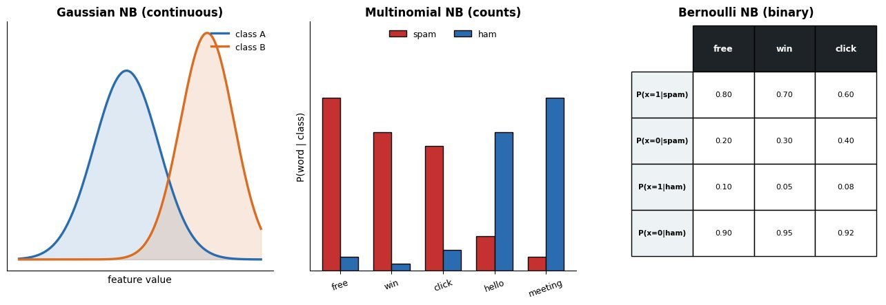
Three panels: Gaussian NB shows bell curves per class for a continuous feature; Multinomial NB shows a bar chart of word count probabilities per class; Bernoulli NB shows a binary presence/absence table with P(x=1|y) and P(x=0|y)

Figure 1: The three Naive Bayes variants: Gaussian models continuous features as per-class normal distributions, Multinomial models count data as a multinomial over a vocabulary, and Bernoulli models binary presence/absence with explicit absence probabilities.

The choice between Multinomial and Bernoulli for text depends on document length and whether absence carries information. Multinomial NB uses word frequencies, so a word appearing three times contributes three times the evidence; Bernoulli NB uses only presence, so “free” appearing once or ten times contributes the same amount, but the absence of “free” also contributes evidence. For long documents where frequency matters (emails, articles), Multinomial is standard. For short documents where presence is the signal (search queries, short reviews), Bernoulli can match or beat Multinomial. A common production pattern is TF-IDF weighting with Multinomial NB, as in the Banking77 support ticket router that classifies 13,000 banking queries into 77 intents in under 1 ms per ticket. For mixed feature types (continuous plus categorical plus binary), scikit-learn does not natively combine variants, so practitioners either discretize continuous features or use the R naivebayes package which supports mixed distributions including kernel density estimation.

Mathematical Formulation:
$P(x_j \mid y) = \frac{1}{\sqrt{2\pi\sigma_{yj}^2}} \exp\!\left(-\frac{(x_j - \mu_{yj})^2}{2\sigma_{yj}^2}\right)$
$P(x_j \mid y) = \frac{N_{yj} + \alpha}{N_y + \alpha\, d}$
$P(x_j \mid y) = \theta_{yj}^{x_j}(1 - \theta_{yj})^{1 - x_j}$

Where:

The first equation is Gaussian NB: $\mu_{yj}$ and $\sigma_{yj}^2$ are the mean and variance of feature $j$ in class $y$ , estimated from training data.
The second equation is Multinomial NB: $N_{yj}$ is the count of feature $j$ in class $y$ , $N_y$ is the total count, $\alpha$ is Laplace smoothing, and $d$ is the vocabulary size.
The third equation is Bernoulli NB: $\theta_{yj} = P(x_j = 1 \mid y)$ is the probability that feature $j$ is present in class $y$ ; the term $(1 - \theta_{yj})^{1 - x_j}$ explicitly models the absence of the feature.

Variant	Feature Type	Distribution	Best For
Gaussian NB	Continuous (real-valued)	Normal per class	Medical diagnosis, sensor data, Iris dataset
Multinomial NB	Counts or TF-IDF	Multinomial	Email spam, review classification, ticket routing
Bernoulli NB	Binary presence/absence	Bernoulli	Short text, boolean features, spam with word presence

August 12, 2026

ML0090 Naive Bayes Classifier

Explain the Naive Bayes classifier and the “naive” conditional independence assumption behind it, as used in production spam detection and support ticket routing.

Answer

Naive Bayes is a probabilistic classifier that applies Bayes’ theorem with a “naive” assumption: given the class label, all features are conditionally independent. This lets the classifier multiply per-feature likelihoods instead of estimating the full joint distribution, which would require exponential data. Despite the assumption being almost always violated in practice, Naive Bayes trains in O(nd) time, predicts in O(d) time, and performs surprisingly well on text classification, spam filtering, and support ticket routing. A production case study processes 85,000 product reviews per day with Multinomial Naive Bayes, achieving AUC above 0.99 for spam detection while retraining in under 5 minutes on a single-core VM, and a TF-IDF plus Multinomial NB pipeline routes banking support tickets in under 1 millisecond per ticket on the Banking77 dataset.

(1) Bayes’ Theorem Applied: the classifier computes the posterior $P(y \mid x)$ for each class and picks the argmax; the naive assumption factors the likelihood $P(x_1, \ldots, x_d \mid y)$ into a product of one-dimensional terms $\prod P(x_j \mid y)$ .
(2) Why the Assumption Works Anyway: even when the independence assumption is wrong, the argmax decision is often correct because correlated features push the posterior in the same direction; the calibration is off but the ranking is not, which is why scikit-learn recommends CalibratedClassifierCV with isotonic regression for reliable probabilities.
(3) Production Strengths: trains in milliseconds, predicts in microseconds, needs no GPU, produces interpretable per-feature contributions, and a 2024 Generalized Naive Bayes paper showed that relaxing the independence assumption via optimal structure learning improves accuracy while keeping the computational profile.

Two panels: left shows the full joint distribution P(x1,x2,x3|y) as a large table requiring exponential data; right shows the naive factorization as three small per-feature tables P(x1|y), P(x2|y), P(x3|y) multiplied together

Figure 1: The naive independence assumption factorizes the intractable joint likelihood P(x1, x2, x3 | y) into a product of one-dimensional per-feature likelihoods, replacing an exponential-size table with d small tables.

The independence assumption is the single most important thing to understand about Naive Bayes, because it is both its source of speed and its source of error. When two features are highly correlated (e.g., “free” and “gift” both appearing in spam), the classifier double-counts their evidence, pushing the posterior toward 0 or 1 more aggressively than the true joint distribution would. This is why GaussianNB in scikit-learn tends to produce overconfident probabilities and why calibration is recommended. The assumption also means Naive Bayes cannot capture feature interactions; a 2024 paper on Generalized Naive Bayes (GNB) addresses this by learning an optimal dependency structure among features while preserving the efficient factorization, proving the approximation is at least as good as classical Naive Bayes. For text specifically, the classic remedies are TF-IDF weighting, document-length normalization, and complement Naive Bayes, introduced by Rennie et al. to correct the multinomial model’s mismatch with real text. In practice, the speed-accuracy trade-off favors Naive Bayes for high-volume, low-latency text tasks where a transformer would be overkill.

Mathematical Formulation:
$\hat{y} = \arg\max_{y}\; P(y) \prod_{j=1}^{d} P(x_j \mid y)$
$P(x_j \mid y) = \frac{N_{yj} + \alpha}{N_y + \alpha\, d}$

Where:

$\hat{y}$ is the predicted class; $P(y)$ is the class prior, and the product of per-feature likelihoods replaces the intractable joint $P(x_1, \ldots, x_d \mid y)$ under the naive conditional independence assumption.
The second equation is the smoothed estimator for discrete (count) features: $N_{yj}$ is the count of feature $j$ in class $y$ , $N_y$ is the total count for class $y$ , $d$ is the vocabulary size, and $\alpha$ is the Laplace smoothing parameter (typically 1) that prevents zero probabilities for unseen feature-class combinations. Continuous features use a density instead, such as a per-class Gaussian.
The argmax is computed in log space to avoid underflow: $\log P(y) + \sum_j \log P(x_j \mid y)$ , which is a sum of precomputed log-likelihoods and runs in O(d) per prediction.

Property	Naive Bayes	Logistic Regression
Training Cost	O(nd) single pass	O(nd) per iteration, multiple iterations
Key Assumption	Conditional independence of features given class	No independence assumption; linear decision boundary
Calibration	Overconfident; needs isotonic calibration	Well-calibrated by default
Interpretability	Per-feature log-likelihood contributions	Per-feature weights (coefficients)
Best For	High-volume text, spam, ticket routing	General tabular classification with calibrated probabilities

August 12, 2026

ML0089 Hidden Markov Model

What is a Hidden Markov Model, and what are its three fundamental problems?

Answer

A Hidden Markov Model is a doubly stochastic generative model for sequential data: a hidden state sequence evolves as a first-order Markov chain (each state depends only on the previous one), and each state emits an observable symbol according to a state-specific distribution. The model is defined by three quantities: the initial state distribution, the transition matrix between states, and the emission distributions. The three fundamental problems are evaluation (what is the probability of an observation sequence), decoding (what is the most likely state sequence given the observations), and learning (how to estimate the parameters from data). In production, DNN-HMM hybrids remain common for on-device keyword spotting, where the DNN estimates emission probabilities and the HMM’s Viterbi decoder integrates across frames, while profile HMMs (Pfam, HMMER) remain the standard for protein family classification across sequenced genomes.

(1) Evaluation (Forward Algorithm): given model parameters and an observation sequence, compute the total probability efficiently via dynamic programming in O(TN^2) instead of summing over all N^T possible state paths.
(2) Decoding (Viterbi Algorithm): find the single most likely state sequence via dynamic programming with backpointers, also O(TN^2); on-device keyword spotters use Viterbi to combine per-frame DNN scores into a detection decision.
(3) Learning (Baum-Welch / EM): estimate transition and emission parameters from unlabeled observation sequences using the forward-backward algorithm, an instance of EM that iterates between computing expected state occupancies (E-step) and updating parameters (M-step); profile HMM databases like Pfam build models from seed alignments and HMMER scores new sequences against them for genome annotation.

HMM architecture: hidden states s1 through s4 connected by transition arrows in a chain, each state emitting an observation o1 through o4 from its emission distribution, with the Markov property annotated

Figure 1: HMM architecture: hidden states form a first-order Markov chain (transitions depend only on the previous state), and each state emits an observation from its own distribution; only observations are visible, states are hidden.

In production, HMMs persist where their probabilistic sequence structure and low computational cost outweigh the accuracy advantage of end-to-end neural models. On-device voice triggers run DNN-HMM hybrids on low-power processors because the HMM’s Viterbi decoder integrates frame-level DNN scores into a keyword hypothesis with minimal power. GMM-derived i-vectors are still fed to DNN-HMM acoustic models as speaker-adaptation features, yielding 5-7% relative WER improvement. In bioinformatics, profile HMMs remain dominant: Pfam 38 (2025) uses HMMER for protein family classification across all sequenced genomes, and the HAVAC FPGA accelerator (2024) speeds up HMMER’s ungapped-Viterbi (SSV) filter stage by as much as 60x. In finance, HMMs are actively used for market regime detection, often hybridized with reinforcement learning for portfolio management.

Three panels: evaluation shows forward recursion summing over previous states; decoding shows Viterbi keeping only the best previous path with backpointers; learning shows Baum-Welch iterating between expected state counts and parameter updates

Figure 2: The three fundamental HMM problems: evaluation (forward algorithm sums over all paths), decoding (Viterbi keeps the single best path via backpointers), and learning (Baum-Welch iterates E-step expected counts with M-step parameter updates).

Mathematical Formulation:
$\alpha_t(j) = \left[\sum_{i=1}^{N} \alpha_{t-1}(i)\, a_{ij}\right] b_j(o_t)$
$\delta_t(j) = \max_{i} \big[\delta_{t-1}(i)\, a_{ij}\big]\, b_j(o_t)$
$\gamma_t(i) = \frac{\alpha_t(i)\, \beta_t(i)}{\sum_{j} \alpha_t(j)\, \beta_t(j)}$

Where:

$\alpha_t(j)$ is the forward variable: the joint probability of emitting $o_1, \ldots, o_t$ and landing in state $j$ at time $t$ ; the evaluation problem sums $\alpha_T(j)$ over all final states.
$\delta_t(j)$ is the Viterbi variable: the highest probability of any single path ending in state $j$ at time $t$ ; backpointers $\psi_t(j)$ record the argmax to reconstruct the best path.
$\gamma_t(i)$ is the posterior state occupancy, formed from the forward variable and the backward variable $\beta_t(i)$ , the probability of emitting the remaining observations $o_{t+1}, \ldots, o_T$ given state $i$ at time $t$ .
$a_{ij}$ is the transition probability from state $i$ to state $j$ and $b_j(o_t)$ the emission probability of $o_t$ in state $j$ . Baum-Welch updates $a_{ij}$ and $b_j$ using $\gamma_t$ and the pairwise posterior $\xi_t(i,j)$ .

Problem	Algorithm	Complexity	Production Use
Evaluation	Forward algorithm	O(TN^2)	Scoring sequences against Pfam profile HMMs
Decoding	Viterbi algorithm	O(TN^2)	On-device keyword spotting (DNN-HMM)
Learning	Baum-Welch (EM)	O(TN^2) per iteration	Training Pfam profile HMMs from seed alignments

August 12, 2026

ML0071 Covariance vs Correlation

What is the difference between covariance and correlation?

Answer

Both measure how two variables move together. Covariance is the raw co-movement, expressed in the product of the two variables’ units: positive when the variables tend to sit above their means together, negative when one runs high while the other runs low. Correlation (Pearson’s $\rho$ ) is covariance divided by both standard deviations, which strips the units and bounds the result to $[-1, 1]$ , so strengths become comparable across datasets. Neither proves causation, and both capture only linear association: a perfect parabola scores zero correlation despite being fully determined.

(1) Units: covariance keeps the product of the units (dollars times kilograms); correlation is unitless and bounded, so rescaling a variable changes the covariance but leaves the correlation untouched.
(2) Sign vs Strength: covariance tells you the direction of co-movement; only correlation tells you a comparable strength, since $0.9$ vs $0.2$ means the same thing for any pair of variables.
(3) Linear Only: both are second-moment statistics of linear association. Zero correlation does not imply independence: $Y = X^2$ on symmetric data has $\rho = 0$ while $X$ fully determines $Y$ .

Four scatter panels: positive correlation, negative correlation, zero correlation with independent points, and a parabola with zero correlation but full dependence

Figure 1: Correlation reads linear co-movement: positive (top left), negative (top right), zero with independence (bottom left), and the trap case, zero correlation with complete dependence on a parabola (bottom right). The first three have matching covariance signs; the fourth shows why a second-moment statistic can miss structure.

Mathematical Formulation:
$\mathrm{Cov}(X, Y) = \mathbb{E}\big[(X - \mu_X)(Y - \mu_Y)\big]$
$\rho_{XY} = \frac{\mathrm{Cov}(X, Y)}{\sigma_X \, \sigma_Y}$

Where:

$X, Y$ are random variables with means $\mu_X, \mu_Y$ and standard deviations $\sigma_X, \sigma_Y$ .
$\mathbb{E}[\cdot]$ is expectation over the joint distribution; in practice both quantities are estimated by sample averages.
$\rho_{XY}$ lies in $[-1, 1]$ by the Cauchy-Schwarz inequality, with $\pm 1$ meaning an exact linear relationship.

Feature	Covariance	Correlation
Definition	Mean product of centered values	Covariance divided by both $\sigma$
Units	Product of the variables’ units	Unitless
Range	Unbounded	$[-1, 1]$
Scale Invariance	No: rescaling a variable rescales it	Yes: unchanged by a positive affine rescaling (a negative scale flips the sign)
Typical Use	Portfolio variance, covariance matrices, PCA	Comparing association strength, feature screening

August 10, 2026

ML0070 A/B Test Design

How would you design an A/B test, including sample size and duration?

Answer

An A/B test is a randomized controlled trial: randomly assign users to control (A) and treatment (B), measure a pre-registered primary metric, and compare the two arms with a hypothesis test. The design happens before any traffic flows: pick one primary metric and a minimum detectable effect (MDE), fix $\alpha$ and power (0.05 and 0.8 are common defaults), and compute the required sample size per arm from the metric’s variance. Duration follows from daily traffic, rounded up to whole business cycles (at least one to two weeks) so day-of-week effects average out, and the decision is made once at the pre-committed end rather than by peeking at daily p-values.

(1) Hypothesis and MDE First: state the expected effect and the smallest effect worth shipping for. The MDE, $\alpha$ , power, and metric variance together pin down the sample size.
(2) Duration by Cycles, Not by Peeking: run whole weeks to cover weekly seasonality and never stop early on a crossing p-value. Booking.com simulated null experiments and found that daily peeking lets over half of them touch 95% significance at some point, versus the promised 5%.
(3) Sensitivity Is the Bottleneck: variance reduction beats longer runs. CUPED (developed at Microsoft) uses pre-experiment covariates to cut metric variance by about 50%, halving the required users or duration, and Booking.com warns that tracking users the change cannot reach dilutes the measured effect and inflates the required sample size by the dilution factor squared.

Flow diagram: hypothesis with MDE leads to random assignment into arms A and B, then a run of full weekly cycles, then one test at the pre-committed end, then a ship or iterate decision

Figure 1: The design pipeline: fix the hypothesis, MDE, $\alpha$ , and power up front; randomize; run whole business cycles; test exactly once at the pre-committed sample size; then ship, iterate, or abandon.

Mathematical Formulation:
$n = \frac{2 \, (z_{1-\alpha/2} + z_{1-\beta})^2 \, \sigma^2}{\delta^2}$
$\sigma^2 = p \, (1 - p) \ \text{for a binary metric}$

Where:

$n$ is the required sample size per arm; $\delta$ is the MDE; $\sigma^2$ is the per-user metric variance.
$z_{1-\alpha/2}$ and $z_{1-\beta}$ are normal quantiles for the significance level and power (1.96 and 0.84 at the usual settings).
$p$ is the baseline rate for a binary metric such as conversion, whose variance is set by $p(1 - p)$ .

Sample size per arm on a log scale falling with the square of the minimum detectable effect, with a marked point at 1 percentage point MDE on a 10 percent baseline needing about 14400 users per arm

Figure 2: Sample size per arm falls with the square of the MDE: halving the detectable effect quadruples the traffic needed. On a 10% conversion baseline, a 1-point MDE needs about 14,400 users per arm; a 0.25-point MDE needs about 230,000.

Decision Rule	When You Look	False Positive Control	Cost
Fixed horizon (pre-committed n)	Once, at the end	Exact $\alpha$	Requires patience
Naive peeking	Daily, stop on significance	Inflated: Booking’s nulls hit 95% over half the time	Ships noise
Sequential test (mSPRT, group-sequential)	Any time	Controlled by construction	Wider confidence sequences

Two histograms of the estimated treatment minus control difference: a wide raw distribution and a narrow CUPED-adjusted distribution centered on the same effect

Figure 3: CUPED regresses out the part of the metric explained by pre-experiment behavior, leaving the same estimated effect with roughly half the variance. That is equivalent to doubling the sample size without adding a single user.

August 10, 2026

ML0069 Z-Test vs T-Test

When do you use a z-test versus a t-test?

Answer

Both tests compare an estimated effect with its standard error to judge whether a mean differs from a reference value. Use a z-test when the reference distribution can be treated as exactly normal: the population standard deviation $\sigma$ is known, or the sample is large enough that the estimate of $\sigma$ is essentially exact. Use a t-test when $\sigma$ is estimated from a small sample: the extra estimation uncertainty fattens the tails of the test statistic, and the t-distribution with $n - 1$ degrees of freedom accounts for it. As $n$ grows, the t-distribution converges to the normal, so beyond a few dozen observations the two tests give nearly identical p-values.

(1) Same Statistic, Different Reference: both divide an effect estimate by its standard error; they differ only in whether the reference distribution is the standard normal or the heavier-tailed t.
(2) When t Is Mandatory: small samples with unknown $\sigma$ , where the t’s heavier tails keep the false positive rate at the promised $\alpha$ . Use Welch’s variant when the two groups have unequal variances.
(3) In Practice at Scale: conversion metrics in online experiments are proportions with millions of users, so the normal (z) approximation is effectively exact; Booking.com’s experimentation write-ups fall back to the two-sample t-test when comparing means on smaller or skewed samples.

Standard normal curve overlaid with a heavy-tailed t distribution with 3 degrees of freedom, the t tails visibly higher beyond plus minus 2

Figure 1: Why the distinction exists: the t-distribution (3 degrees of freedom shown) has visibly heavier tails than the standard normal, so its critical values sit farther out. As degrees of freedom grow, the t curve collapses onto the normal and the two tests coincide.

Mathematical Formulation:
$z = \frac{\bar{x} - \mu_0}{\sigma / \sqrt{n}}$
$t = \frac{\bar{x} - \mu_0}{s / \sqrt{n}}$

Where:

$\bar{x}$ is the sample mean, $\mu_0$ the hypothesized mean, and $n$ the sample size.
$\sigma$ is the known population standard deviation used by the z-test; $s$ is the sample-estimated standard deviation used by the t-test.
The t statistic follows a t-distribution with $n - 1$ degrees of freedom, which approaches $N(0, 1)$ as $n$ grows.

Feature	Z-Test	T-Test
Spread Parameter	$\sigma$ known (or $n$ huge)	$s$ estimated from the sample
Reference Distribution	Standard normal	t with $n - 1$ degrees of freedom
Tail Behavior	Thinner tails, tighter critical values	Heavier tails at small $n$
Typical Case	Proportion tests at scale (conversion)	Small samples, heavy-tailed metrics
Large-n Behavior	Asymptotically valid for proportions via the CLT	Coincides with the z-test

August 10, 2026

ML0068 Type I vs Type II Errors
What are Type I and Type II errors, and how do they trade off?
Answer
A Type I error (false positive) rejects a true null hypothesis: you announce an effect that is not there. A Type II error (false negative) fails to reject a false null: a real effect goes undetected. Their rates are $\alpha$ , the significance level you choose up front, and $\beta$ , with power equal to $1 - \beta$ . For a fixed sample size the two trade off through the decision threshold: making the test stricter lowers $\alpha$ but raises $\beta$ , and only more data or lower metric variance reduces both at once.
(1) Type I ( $\alpha$ ): rejecting a true null, the “convicting the innocent” error. It is controlled by fixing $\alpha$ before looking at data and by correcting when many hypotheses are tested at once.
(2) Type II ( $\beta$ ): missing a real effect. Power $1 - \beta$ grows with sample size, true effect size, and lower metric variance.
(3) Costs Set the Threshold: the right balance is a business decision. Gmail blocks over 99.9% of spam while misrouting only about 0.05% of legitimate mail, because a false positive (lost mail) costs far more than a false negative (spam seen in the inbox).

Figure 1: Sampling distribution of the test statistic under $H_0$ (left) and $H_1$ (right) with one decision threshold. The right tail of $H_0$ is $\alpha$ (Type I), the part of $H_1$ left of the threshold is $\beta$ (Type II), and the rest of $H_1$ is power.
Mathematical Formulation:
$\alpha = \Pr(\text{reject } H_0 \mid H_0 \text{ true})$
$\beta = \Pr(\text{fail to reject } H_0 \mid H_1 \text{ true})$
$\text{power} = 1 - \beta$
Where:
$H_0$ is the null hypothesis (no effect) and $H_1$ the alternative (a real effect exists).
$\alpha$ is the significance level chosen before the test; $\beta$ is the false negative rate under a specific true effect.
Power is the probability of detecting the effect when it is real, and it rises with sample size, effect size, and reduced variance.

Figure 2: Moving the threshold at fixed sample size swaps the errors: stricter (left panel) shrinks $\alpha$ and inflates $\beta$ ; looser (right panel) does the reverse. Shrinking both at once requires more data or lower variance, which pulls the two curves apart.
Decision \ Reality H0 True (No Effect) H1 True (Real Effect)
Reject H0 Type I error, rate $\alpha$ Correct detection, power $1 - \beta$
Fail to Reject H0 Correct, rate $1 - \alpha$ Type II error, rate $\beta$
Login to view more content
August 10, 2026

Decision \ Reality	H0 True (No Effect)	H1 True (Real Effect)
Reject H0	Type I error, rate $\alpha$	Correct detection, power $1 - \beta$
Fail to Reject H0	Correct, rate $1 - \alpha$	Type II error, rate $\beta$