
What are the different types of Naive Bayes classifiers (Gaussian, Multinomial, Bernoulli), and when is each appropriate for tasks like Microsoft’s spam filtering or medical diagnosis?
Answer
The three main variants of Naive Bayes differ in the distribution they assume for each feature given the class, and the choice is driven by the feature type. Gaussian Naive Bayes assumes each continuous feature follows a normal distribution per class, estimated by the class-conditional mean and variance; it suits real-valued features like medical lab values or sensor readings. Multinomial Naive Bayes models integer feature counts drawn from a multinomial distribution, and in practice TF-IDF weights are often substituted even though they are not counts; it is the standard for text classification, used in Microsoft’s spam filtering training module and production review-spam detection processing 85,000 reviews per day. Bernoulli Naive Bayes models binary presence/absence indicators with a Bernoulli distribution; it suits boolean features like “contains word X” or “has flag Y” and explicitly accounts for the absence of a feature, which Multinomial NB does not.
(1) Gaussian NB (Continuous): estimates  and
and  per class per feature; best for real-valued features like blood pressure, age, or sensor readings; assumes normality, so skewed or multi-modal features need transformation or kernel density estimation.
(2) Multinomial NB (Count Data): estimates  ; the standard for text classification on word counts, and commonly run on TF-IDF weights as a practical approximation; Microsoft’s training module uses it for email spam filtering, and a production system classifies 85,000 reviews/day at AUC above 0.99.
(3) Bernoulli NB (Binary Presence): estimates  and explicitly models
  ; best for short documents or boolean feature sets where absence is informative; scikit-learn ships it alongside categorical and complement variants, and the R naivebayes package adds a Poisson variant for count features.
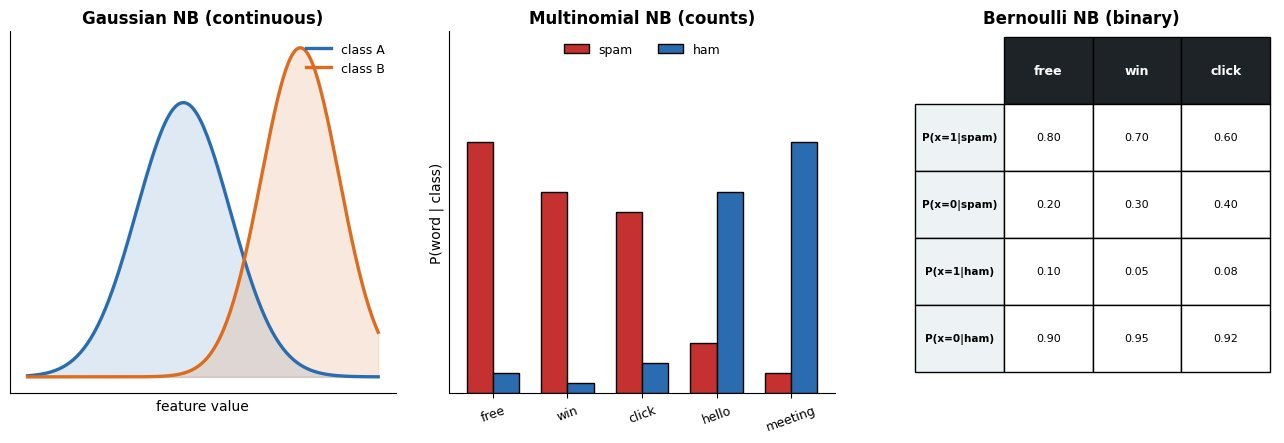
Figure 1: The three Naive Bayes variants: Gaussian models continuous features as per-class normal distributions, Multinomial models count data as a multinomial over a vocabulary, and Bernoulli models binary presence/absence with explicit absence probabilities.
The choice between Multinomial and Bernoulli for text depends on document length and whether absence carries information. Multinomial NB uses word frequencies, so a word appearing three times contributes three times the evidence; Bernoulli NB uses only presence, so “free” appearing once or ten times contributes the same amount, but the absence of “free” also contributes evidence. For long documents where frequency matters (emails, articles), Multinomial is standard. For short documents where presence is the signal (search queries, short reviews), Bernoulli can match or beat Multinomial. A common production pattern is TF-IDF weighting with Multinomial NB, as in the Banking77 support ticket router that classifies 13,000 banking queries into 77 intents in under 1 ms per ticket. For mixed feature types (continuous plus categorical plus binary), scikit-learn does not natively combine variants, so practitioners either discretize continuous features or use the R naivebayes package which supports mixed distributions including kernel density estimation.
Mathematical Formulation:


Where:
- The first equation is Gaussian NB:
 and
and  are the mean and variance of feature
  in class
  , estimated from training data.
 - The second equation is Multinomial NB:
 is the count of feature in class ,
  is the total count,
  is Laplace smoothing, and
  is the vocabulary size.
 - The third equation is Bernoulli NB:
 is the probability that feature is present in class ; the term
  explicitly models the absence of the feature.
 in class
  , estimated from training data.
 is the count of feature
  is the total count,
  is Laplace smoothing, and
  is the vocabulary size.
 is the probability that feature
  explicitly models the absence of the feature.
| Variant | Feature Type | Distribution | Best For |
|---|---|---|---|
| Gaussian NB | Continuous (real-valued) | Normal per class | Medical diagnosis, sensor data, Iris dataset |
| Multinomial NB | Counts or TF-IDF | Multinomial | Email spam, review classification, ticket routing |
| Bernoulli NB | Binary presence/absence | Bernoulli | Short text, boolean features, spam with word presence |
Leave a Reply