
How would you design an A/B test, including sample size and duration?
Answer
An A/B test is a randomized controlled trial: randomly assign users to control (A) and treatment (B), measure a pre-registered primary metric, and compare the two arms with a hypothesis test. The design happens before any traffic flows: pick one primary metric and a minimum detectable effect (MDE), fix  and power (0.05 and 0.8 are common defaults), and compute the required sample size per arm from the metric’s variance. Duration follows from daily traffic, rounded up to whole business cycles (at least one to two weeks) so day-of-week effects average out, and the decision is made once at the pre-committed end rather than by peeking at daily p-values.
(1) Hypothesis and MDE First: state the expected effect and the smallest effect worth shipping for. The MDE, , power, and metric variance together pin down the sample size.
(2) Duration by Cycles, Not by Peeking: run whole weeks to cover weekly seasonality and never stop early on a crossing p-value. Booking.com simulated null experiments and found that daily peeking lets over half of them touch 95% significance at some point, versus the promised 5%.
(3) Sensitivity Is the Bottleneck: variance reduction beats longer runs. CUPED (developed at Microsoft) uses pre-experiment covariates to cut metric variance by about 50%, halving the required users or duration, and Booking.com warns that tracking users the change cannot reach dilutes the measured effect and inflates the required sample size by the dilution factor squared.
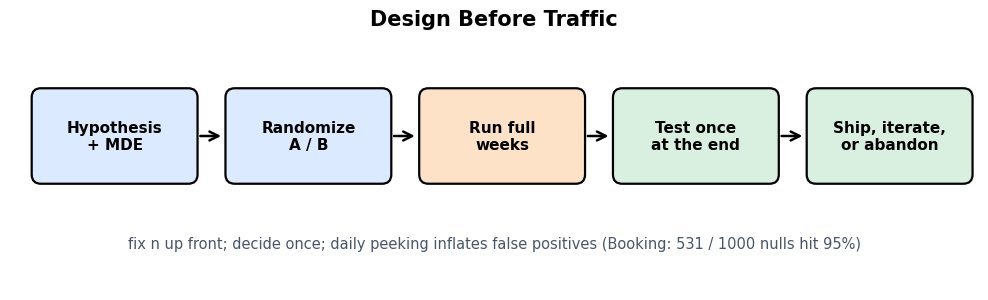
Figure 1: The design pipeline: fix the hypothesis, MDE, , and power up front; randomize; run whole business cycles; test exactly once at the pre-committed sample size; then ship, iterate, or abandon.
Mathematical Formulation:


Where:
 is the required sample size per arm;
  is the MDE;
  is the per-user metric variance.
 and
and  are normal quantiles for the significance level and power (1.96 and 0.84 at the usual settings).
 is the baseline rate for a binary metric such as conversion, whose variance is set by
  .
.
 is the required sample size per arm;
  is the MDE;
  is the per-user metric variance.
 and
and  are normal quantiles for the significance level and power (1.96 and 0.84 at the usual settings).
 is the baseline rate for a binary metric such as conversion, whose variance is set by
  .
.
Figure 2: Sample size per arm falls with the square of the MDE: halving the detectable effect quadruples the traffic needed. On a 10% conversion baseline, a 1-point MDE needs about 14,400 users per arm; a 0.25-point MDE needs about 230,000.
| Decision Rule | When You Look | False Positive Control | Cost |
|---|---|---|---|
| Fixed horizon (pre-committed n) | Once, at the end | Exact | Requires patience |
| Naive peeking | Daily, stop on significance | Inflated: Booking’s nulls hit 95% over half the time | Ships noise |
| Sequential test (mSPRT, group-sequential) | Any time | Controlled by construction | Wider confidence sequences |

Figure 3: CUPED regresses out the part of the metric explained by pre-experiment behavior, leaving the same estimated effect with roughly half the variance. That is equivalent to doubling the sample size without adding a single user.
Leave a Reply