Tag: System

  • MSD0053 Video Chaptering Keyframe

    Design a deep learning system for autonomous video chaptering and keyframe extraction. A video platform (YouTube, Vimeo, Coursera) must automatically segment uploaded videos into chapters and extract representative keyframes so that viewers can navigate to specific sections without scrubbing through the entire video. For a 45-minute lecture, the system must detect topic boundaries (when the speaker moves from “gradient descent” to “backpropagation”), assign a chapter title to each segment, and pick one keyframe per chapter that best represents its content.

    The system must handle diverse video types (lectures, vlogs, tutorials, interviews, gameplay) with no manual metadata, detect both visual and audio scene changes (a slide change, a speaker cut, a topic shift in the transcript), and produce chapter titles that are concise and informative. The system must process hundreds of thousands of uploaded videos per day, and the chaptering must be good enough that viewers prefer the auto-generated chapters over no chapters at all.

    How would you design this system? Cover the multimodal feature extraction (visual embeddings from frame sampling, audio features, transcript text), the boundary detection model (shot boundary detection vs topic segmentation vs learned segmentation), the keyframe selection strategy (clustering vs diversity sampling vs attention-based), the chapter title generation approach (extractive from transcript vs abstractive summarization vs LLM generation), and how you evaluate chaptering quality when there is no ground truth for most videos.

    Line-art scene: a viewer reaching for the scrub bar under a long film strip of lecture frames, transcript snippets about gradient descent and backpropagation on either side of a question mark, and a stack of uploads arriving at the right

    The Problem: a 45-minute video arrives as raw frames and audio with no table of contents. Find where each topic starts, name it, and pick the one frame that stands for it, for hundreds of thousands of uploads a day.

    Answer

    The design is an upload-time batch pipeline that turns every video into a per-second sequence of multimodal tokens (frame embeddings with OCR text, speaker-change and music cues from the audio, sentence embeddings from the ASR transcript) and runs a learned boundary transformer over that sequence to predict where chapters start. Shot-boundary detection and transcript topic segmentation are input features to this model rather than the model itself, so a slide flip alone does not cut a chapter while a topic shift inside one static shot still does. The model is trained on creator-supplied chapter timestamps, the millions of videos where creators already typed chapters into the description, filtered to remove noisy chaptering. Each chapter then receives a keyframe chosen as the quality-filtered medoid of its frame embeddings and a title written by an instruction-tuned LLM that reads the chapter’s transcript and slide text under a grounding check, with an extractive fallback. Quality is proven the way the product will be judged: tolerance-window F1 against creator chapters, pairwise human ratings, and online navigation behavior.

    (1) One Time Axis: resample every modality to one token per second so boundaries, keyframes, and titles share coordinates; a 45-minute lecture becomes 2,700 tokens.
    (2) Weak Labels from Creators: train on creator timestamps that satisfy the platform’s chapter rules (at least three chapters, each 10 s or longer, first at 0:00), reweighted by video type and held out by creator.
    (3) Learned Boundary Model over Signals: shot cuts, speaker changes, and transcript cohesion dips are features; a transformer outputs P(boundary at t) and decoding enforces a minimum chapter length.
    (4) Quality-Filtered Medoid Keyframe: discard blurry, dark, and transition frames near boundaries, then pick the medoid frame, the one that minimizes total distance to every other frame in the chapter.
    (5) Grounded LLM Titles: generate 2-6 word titles from the transcript plus OCR text in one call per video; reject titles whose content words never appear in the source and fall back to the top extractive phrase.
    (6) Evaluation Without Truth: tolerance-window boundary F1 on creator-chaptered holdouts, pairwise raters, and chapter click and seek metrics online; withhold chapters when confidence is low.

    Chaptering pipeline: an uploaded video fans out into visual, audio, and transcript feature streams that merge in a per-second boundary transformer; chapter spans feed a keyframe selector and a title generator, which assemble the chapter index, while creator edits and viewer navigation logs flow back as training signal

    Figure 1: The chaptering pipeline: three feature streams on one time axis, one learned boundary model, then keyframe and title stages per chapter, with creator edits and navigation logs feeding retraining.

    Clarify Before Designing:
    (1) Content Mix and Length: what share of uploads is speech-dense (lectures, interviews) versus gameplay, music, or silent screen recordings, and what does the duration tail look like (multi-hour stream replays)?
    (2) Freshness Budget: must chapters exist at publish time, or is a delay of minutes to an hour acceptable, and may we reprocess the back catalog when the model improves?
    (3) Existing Signals: does the platform already run ASR for captions, and does it store creator-typed chapter timestamps that can serve as labels?
    (4) Product Constraints: minimum and maximum chapter counts, minimum chapter length, title length cap, and whether creators can edit or disable auto chapters?
    (5) Cost Envelope: how many GPU-hours per thousand video-hours are allowed, which decides frame sampling rate, ASR model size, and whether an LLM runs per video?
    (6) Language Coverage: which languages need titles, and how reliable is the transcript for each?


    Login to view more content
  • MSD0052 Airbnb Photo Tagging

    Design a system that automatically tags photos uploaded by hosts (e.g., “kitchen”, “bedroom”, “pool”, “ocean view”) on Airbnb using a deep image classification model. When a host creates or edits a listing, they upload dozens of photos, and Airbnb must automatically label each photo with the room type or amenity it depicts so that guests can filter by feature (“pool”, “mountain view”) and the listing page can organize photos into structured sections (Living Room, Bedroom, Kitchen, Exterior). The system must handle a wide taxonomy of tags (50+ room types and amenities), work across varying photo quality, angles, and lighting from phone cameras worldwide, distinguish similar categories (“living room” vs “family room”, “balcony” vs “patio”), and handle the long tail of rare amenities (“sauna”, “wine cellar”) that have few training examples. Mislabeling a bathroom as a kitchen degrades search relevance and user trust, so the system must flag low-confidence tags for host confirmation rather than auto-assigning them.

    How would you design this system? Cover the classification model architecture (single-label vs multi-label vs hierarchical classification), how you handle the long tail of rare tags with few training examples, how you generate training labels from host-provided metadata and guest clicks, how you calibrate confidence for the host-confirmation workflow, the inference pipeline for processing photo uploads in real time, and how you evaluate tagging accuracy across the full tag taxonomy.

    Line-art scene: a host holding a phone uploads a stack of photos, a magnifier hovers over a corner asking living room or family room, a question mark leads to a column of tag badges (kitchen, bedroom, pool, ocean view) with faded rare tags sauna and wine cellar off to the side

    The Problem: Thirty phone photos arrive per listing and each must land on one of fifty-plus tags, where the popular tags have millions of examples, the rare ones have a few hundred, and a confident wrong tag costs more trust than no tag at all.

    Answer

    The design is a shared vision backbone with two heads: a hierarchical softmax head for the mutually exclusive room or scene type, and a multi-label sigmoid head for amenities that co-occur in one photo. Training labels are mined at scale from host captions, existing photo-section placement, and guest filter clicks, then sharpened by the host confirmations the product itself generates. Rare tags are handled by decoupling representation from classifier: the backbone learns from the head-heavy data, the classifier heads are re-balanced, and tags with too few examples are served through a nearest-prototype path until they graduate. Every prediction passes a per-tag calibrated confidence gate with three outcomes: auto-assign, a one-tap host confirmation card, or leave untagged. Inference runs as a batched GPU service triggered by the upload event, so a 30-photo listing is tagged before the host finishes the flow, and every confirmation flows back into the next training round.

    (1) Label Structure: a scene tree (indoor, outdoor, view) with roughly 40 leaves under a hierarchical softmax, plus roughly 30 amenity tags under independent sigmoids; sibling pairs humans confuse (“living room” vs “family room”) share one merged leaf until a reliable cue separates them.
    (2) Weak Labels at Scale: host captions, section placement, listing-level amenity declarations, and guest clicks after filtering by an amenity give millions of noisy labels; host confirmations and removals form the small gold layer that drives thresholds and evaluation.
    (3) Long Tail by Decoupling: train the backbone on all data, then re-fit the classifier heads with class-balanced sampling and logit adjustment; tags below about 5k labels use a prototype classifier on frozen embeddings.
    (4) Calibrated Confidence Gate: temperature scaling per head and per-tag thresholds tuned on the confirmed holdout to a 98% precision floor; high confidence auto-assigns, the gray zone asks the host, low confidence stays untagged.
    (5) Async GPU Serving at Upload: an upload event triggers fetch, dedupe, batch inference, and a write to a versioned tag store that feeds search filters and section layout; the catalog backfill is a batch job on the same model.
    (6) Confirmation Feedback Loop: confirmations, removals, and re-sectioning are logged as labels with model version, and monthly retraining passes per-region and per-tag gates before release.

    Photo tagging pipeline: host upload flows through preprocessing into a shared backbone that feeds a scene head and an amenity head, both scored by a calibrated confidence gate that either auto-assigns tags to sections and filters or sends a one-tap host confirmation card; a dashed feedback path carries confirmations into the training-label store that retrains the backbone

    Figure 1: One backbone pass per photo, two heads, one gate: confident tags ship, doubtful ones become a host card, and every host answer becomes a training label.

    Clarify Before Designing:
    (1) Taxonomy Ownership: is the 50-tag list fixed or does the product team add tags quarterly, and does a hierarchy (room vs amenity vs view) already exist?
    (2) Latency Expectation: must tags appear inside the upload flow within seconds, or only before the listing goes live minutes later?
    (3) Label Sources: what fraction of photos carry a host caption or a section placement, and are guest filter-and-click logs joinable to individual photos?
    (4) Error Asymmetry: which hurts more, a missing “pool” or a false “pool”, and is there a precision floor the search team already enforces?
    (5) Scale: photos uploaded or edited per day, catalog size for a backfill, and the share of phone versus professional photos?
    (6) Confirmation Budget: how many confirmation prompts per upload before hosts disengage, and may a listing publish while tags are pending?


    Login to view more content
  • MSD0051 Street View Face Blurring

    Design the face and license-plate blurring system for Google Street View using a deep object detection model. Street View captures panoramic street-level imagery from cameras mounted on cars, trekkers, and drones, covering millions of miles of roads across 100+ countries. Every captured panorama must be processed to blur all human faces and vehicle license plates before publication, to comply with privacy laws (GDPR in Europe, CCPA in California, and local regulations worldwide). The system must detect faces and plates at varying scales, angles, lighting, and occlusion (a face in a car window, a plate partially covered by snow), process millions of panoramas per day with minimal compute cost, and keep the false-negative rate near zero because a single unblurred face is a privacy violation. At the same time, false positives that blur non-face objects (signs, manhole covers, building facades) degrade image quality and user experience.

    How would you design this system? Cover the detection model architecture (single-stage detector vs two-stage detector vs segmentation-based), how you handle the extreme scale variation and small objects, how you generate and augment training data for rare cases (motorcycle plates, faces in helmets), how you balance the false-negative vs false-positive trade-off given the privacy-first requirement, the inference pipeline for processing millions of panoramas per day, and how you monitor and audit blur quality at scale.

    Line-art street scene: a capture car with a 360 camera mast drives past pedestrians, a parked car with a license plate, a round road sign and a manhole cover, with annotations for millions of panoramas per day, 100+ countries, and zero unblurred faces allowed, plus a question mark

    The Problem: every panorama hides a handful of faces and plates at 20 to 200 pixels among signs and facades that look like them; miss one and it is a privacy violation, blur too many and the street turns to mush.

    Answer

    The design is a recall-first single-stage detector run on overlapping tiles of the full-resolution panorama, feeding a fail-closed blur gate that no image can bypass on its way to publication. An FPN-style anchor-free detector with separate face and plate heads scores every 1024 px tile at native resolution, detections are merged with panorama-level NMS, and the threshold is set far below the mAP-optimal point so recall, not precision, is what the model is tuned for. Boxes are dilated before blurring, low-confidence boxes go to a cheap verifier that promotes rather than vetoes, and a stratified human audit plus the user report path close the loop on the misses no model catches. The pivotal calls are tiling instead of downscaling, an explicit blur budget instead of a precision target, and treating the blur job as a publication gate rather than a post-processing step.

    (1) Tiled Native-Resolution Input: the 8k by 4k panorama is cut into overlapping 1024 px tiles so a 20 px face is still 20 px when the detector sees it; a 2x upsampled re-crop handles the smallest bucket.
    (2) Single-Stage FPN Detector: an FCOS-class anchor-free model with focal loss, separate face and plate heads, and pyramid levels matched to the 16 to 256 px object range.
    (3) Recall-First Operating Point: the threshold is chosen from the recall-versus-false-positives-per-panorama curve, with a blur budget (blurred pixel fraction) as the only cap on precision loss.
    (4) Blur If In Doubt: boxes are dilated 15 to 20%, overlapping boxes are unioned, and an uncertain band is re-scored by a crop verifier that can add blur but never remove a confident detection.
    (5) Targeted Data Program: country-stratified plate labels, hard-negative mining on facades and signs, and copy-paste augmentation for motorcycle plates, helmets, masks, and faces behind glass.
    (6) Fail-Closed Batch Gate: a panorama publishes only with a signed blur receipt; stratified human audit and user reports feed misses and false blurs back into retraining.

    Blurring pipeline: a stitched panorama is tiled at multiple scales, a single-stage FPN detector with face and plate heads scores tiles, detections are merged with panorama-level NMS, a recall gate applies a low threshold and dilates boxes, uncertain boxes go to a verifier, and the blur and publish stage is fail-closed; a human audit loop feeds hard negatives and missed faces into retraining

    Figure 1: The publication path: tile, detect, merge, blur generously, and never publish without a blur receipt; the audit loop underneath is what keeps recall honest over time.

    Clarify Before Designing:
    (1) Scale and Latency: how many panoramas per day and how many pixels each; is publication latency hours or days, which decides whether this is a batch system or a streaming one?
    (2) Legal Bar: which jurisdictions and what counts as a face or plate (statues, posters, reflections, partial plates), and is “near zero” a measured audit rate or a contractual guarantee?
    (3) Blur Budget: what fraction of blurred non-target pixels per panorama is acceptable before image quality complaints outweigh privacy gains?
    (4) Capture Fleet: how many camera generations and platforms (car, trekker, drone) with different resolutions and viewpoints must one model serve?
    (5) Data Assets: do labeled faces and plates from earlier campaigns exist, and can already-published blurred imagery be reused as training signal?
    (6) Back-Catalog: must a better model reprocess years of published imagery, which changes the compute plan and the rollout policy?


    Login to view more content
  • MSD0050 Document QA Extraction

    Design a question-answering system that extracts an answer from a large document collection given a user query using a deep reading comprehension model. A legal or enterprise search product must let users ask natural-language questions (“What is the termination clause in the NDA?”, “What were the Q3 revenue figures for the EMEA region?”) and return exact answer spans extracted from a corpus of millions of documents: contracts, filings, internal wikis, emails.

    The system must first retrieve the relevant documents or passages from the corpus (the retrieval stage), then run a reading comprehension model over the retrieved passages to extract the answer span (the reader stage), and finally rank or aggregate answers when multiple passages produce candidates. The retrieval stage must handle lexical mismatch (the query says “termination” but the document says “cancellation”), the reader must handle multi-hop reasoning where the answer requires combining information from two passages, and the system must say “I don’t know” when no passage contains a confident answer rather than hallucinating.

    How would you design this system? Cover the retriever architecture (sparse BM25 vs dense bi-encoder vs hybrid retrieval), the reader architecture (extractive span prediction vs generative reading comprehension vs T5/BART-style seq2seq), how you handle multi-hop questions, how you calibrate confidence for abstention, and how you evaluate end-to-end QA accuracy (exact match, F1, answerability detection).

    Line-art scene: a person asks about the termination clause in an NDA, a question mark stands between them and three tall stacks of contracts, filings, wikis and emails, and a magnifier over one page reveals the word cancellation instead of termination

    The Problem: one natural-language question, ten million documents that rarely use the asker’s words, and a product that must quote the exact sentence or admit it cannot find one.

    Answer

    The design is a retrieve-rerank-read pipeline with an explicit abstention gate. A hybrid retriever (BM25 plus a dense bi-encoder, merged by reciprocal rank fusion) pulls about 100 passages from a permission-filtered index, a cross-encoder reranker keeps the top 10, and an extractive reader with a no-answer head scores candidate spans in each passage. Spans are aggregated across passages, and a calibrated confidence threshold decides between returning a cited span and answering “I don’t know”. Multi-hop questions run the same loop twice: the first hop’s reader output becomes a bridge entity that rewrites the query for a second retrieval. The pivotal decisions are hybrid rather than pure dense retrieval (synonyms and exact identifiers both matter in legal and financial text), extractive rather than generative reading (verbatim spans with citations are the product, and a span cannot hallucinate), and a threshold set on the risk-coverage curve rather than on a raw softmax.

    (1) Passage Index with Metadata: split documents into 200-300 token passages with overlap, and store document type, date, region, and access-control lists alongside both the inverted index and the ANN index so filters apply at retrieval time.
    (2) Hybrid Retrieval: BM25 catches exact identifiers (clause numbers, “Q3”, “EMEA”) while the dense bi-encoder catches paraphrase (“termination” versus “cancellation”); reciprocal rank fusion merges both lists into a top-100.
    (3) Cross-Encoder Reranker: joint query-passage encoding narrows 100 → 10 passages and is the largest single quality gain per millisecond in the pipeline.
    (4) Extractive Reader with Null Head: start and end logits plus a no-answer score per passage; identical spans from different passages pool their probability.
    (5) Iterative Multi-Hop: when hop one yields a bridge entity but no final answer, the query is rewritten and retrieval runs again, capped at two hops to bound latency.
    (6) Calibrated Abstention: the null-versus-span margin threshold is chosen on the risk-coverage curve at the product’s tolerated error rate, and abstentions fall back to classic search or a human.

    Document QA pipeline: a permission-filtered query fans out to a BM25 index and a dense ANN index, the lists are fused by RRF into a top-100, a cross-encoder reranker keeps ten, an extractive reader with a null head scores spans, an aggregation and calibration stage emits either a cited answer span or I don't know, and a dashed multi-hop loop feeds the bridge entity back into the query

    Figure 1: The retrieve-rerank-read path with its two exits, a cited span or an honest abstention, and the dashed multi-hop loop that rewrites the query with a bridge entity.

    Clarify Before Designing:
    (1) Corpus and Freshness: how many documents and pages, in which languages and formats (scanned PDFs need OCR), and how quickly must a new filing become searchable?
    (2) Load and Latency: queries per day, acceptable p95 latency for an interactive answer, and whether a slower two-hop path is tolerable for a minority of questions?
    (3) Answer Form: is the product a verbatim span with a citation, or a synthesized paragraph; may the system quote two passages for one answer?
    (4) Multi-Hop Share: what fraction of real questions need two passages, and is a bridge through an entity (a counterparty, a region, a fiscal quarter) the dominant pattern?
    (5) Labels: do in-domain question-answer pairs exist (support tickets, FAQ pages, past research memos), and what annotation budget do domain experts have?
    (6) Error Asymmetry and Access: how much worse is a confidently wrong clause than “I don’t know”, and must answers respect per-user document permissions?


    Login to view more content
  • MSD0047 Robinhood Trading Fraud Detection

    Design Robinhood’s real-time trade monitoring system that analyzes order book activity to identify spoofing, wash trading, and insider trading patterns. A retail brokerage must monitor millions of orders per day in real time, detecting manipulative patterns the moment they form so that offending accounts can be flagged, restricted, or reported to regulators (SEC, FINRA).

    Spoofing means placing large orders with no intent to execute, solely to move the price, then canceling them. Wash trading means an account trading with itself to create fake volume. Insider trading means unusual trading activity correlated with material non-public information. Each pattern has a distinct signature in the order book, but the signals are noisy, the patterns evolve as manipulators adapt, and false positives that freeze legitimate accounts damage trust and invite regulatory scrutiny.

    How would you design this system? Cover the real-time order book feature engineering, the detection model architecture for each manipulation pattern, how you handle the adversarial evolution of manipulation tactics, the alerting and human-review workflow, and how you measure detection precision and recall when confirmed manipulation labels are scarce.

    Line-art scene with three panels: an order book ladder with a huge order that is placed and canceled, two accounts trading back and forth with each other, and a timeline where one account buys days before a news announcement

    The Problem: three very different manipulation signatures hide inside tens of millions of daily order events, and each one has to be recognized while it is still forming.

    Answer

    The design is a streaming surveillance pipeline with one detector per manipulation pattern on top of a shared order-lifecycle feature layer. Every order event (new, modify, cancel, fill) lands in an append-only log, a stateful stream processor maintains per-account and per-symbol rolling features, and three specialized models consume them: a sequence model for spoofing and layering, a graph model over the account-to-account fill network for wash trading, and a retrospective event-study anomaly detector for insider trading. A fusion layer ranks candidates and thresholds them against actual analyst capacity, not against a fixed probability. The two pivotal decisions are to treat scarce labels as a modeling problem in their own right (weak supervision, positive-unlabeled learning, injected synthetic manipulation for recall estimation) and to keep probabilistic models out of the pre-trade order path, where only deterministic checks such as self-trade prevention belong.

    (1) Shared Order-Lifecycle Features: compute cancel-to-fill ratio, order lifetime, depth added within N ticks, book imbalance, and contra-side fill proximity once per event and reuse them across all detectors.
    (2) One Detector Per Pattern: the three signatures live in different data structures (temporal sequences, an account graph, price residuals around news), so a single “manipulation” classifier would blur them and lose explainability.
    (3) Label-Scarce Learning: a few dozen confirmed cases cannot train a supervised model alone, so combine weak supervision from analyst dispositions and regulatory case patterns with an anomaly floor that catches novel tactics.
    (4) Capacity-Calibrated Tiering: thresholds are set so that the daily alert volume matches reviewer throughput, with only the highest-precision deterministic patterns eligible for automated restriction.
    (5) Adversarial Maintenance: champion-challenger models, red-team simulation of evasion (order splitting, cross-account layering), and drift monitors on the feature distributions manipulators can move.
    (6) Auditability By Construction: every alert is reproducible from the immutable event log with a feature snapshot and reason codes, because a FINRA inquiry asks why a specific account was flagged on a specific day.

    Surveillance pipeline: order events, market data and account identity feed a streaming feature layer, which fans out to a spoofing sequence detector, a wash-trade graph detector and an insider anomaly detector; a risk fusion and tiering block routes to an analyst queue, regulator filings and automated restrictions, with a dashed feedback path into a label store and retraining

    Figure 1: One feature layer, three pattern-specific detectors, one capacity-calibrated queue, and a feedback loop that turns analyst dispositions back into labels.

    Clarify Before Designing:
    (1) Regulatory Scope: which patterns are we obligated to surveil, and does the output feed formal reporting (SAR, SRO referral) or only internal risk decisions?
    (2) Intervention Point: must we block a manipulative order before it reaches the venue, or is flagging within seconds after the fact acceptable?
    (3) Data Reach: do we see only our own order flow, or consolidated cross-venue data, since a spoofer can place the phantom side elsewhere?
    (4) Label Supply: how many confirmed cases exist historically, and do regulators tell us whether a referral was substantiated?
    (5) Review Capacity And Cost Asymmetry: how many alerts per day can analysts actually clear, and what is the cost of freezing a legitimate account versus missing a spoof?
    (6) Account Universe: retail only, or also market makers and institutions whose high cancel ratios are entirely legitimate?


    Login to view more content
  • MSD0045 Theme Park Wait Prediction

    A large theme park app (think Disneyland or Universal Studios) must show an accurate wait time for every attraction and forecast it 15 to 60 minutes ahead, so a guest can decide whether to walk across the park now or after lunch. The system ingests real-time signals: ride throughput counters, queue-length estimates from cameras or Bluetooth beacons, ride downtime events, weather, and live park attendance.

    It must learn the patterns that drive wait fluctuations (time of day, day of week, season, holidays, parades and special events) and survive the non-stationarity caused by breakdowns, capacity changes, and brand-new rides. Predictions must update within seconds of a status change, and the app must show a range rather than a single number, because one estimate that is 20 minutes wrong destroys trust in every other number on the screen.

    How would you design this system? Cover the real-time feature ingestion pipeline, the forecasting model architecture (sequence model vs temporal graph vs hybrid), how you handle downtime events and non-stationarity, how you produce calibrated uncertainty intervals, and how you evaluate both prediction accuracy and freshness.

    Line-art scene: a queue of guests under a sign posting 45 minutes while the real wait is 70, a breakdown notice above the ride running two of three trains, rain forecast, park attendance annotation, and a question mark asking what the wait will be in 30 minutes

    The Problem: the posted number is a lagging measurement, while the guest needs a forecast that already accounts for the breakdown, the lost train, the rain, and the crowd walking over right now.

    Answer

    The design is a physics-anchored hybrid forecaster served from a streaming feature pipeline. A queueing-theory baseline gives the mechanical wait from live queue length and boarding throughput, and a learned model predicts the residual plus the multi-horizon trajectory. The learner is a spatiotemporal hybrid: a temporal encoder over each ride’s recent history, message passing over a park graph whose edges encode walking time and historical guest flow, and global context (attendance, weather, event calendar) injected as conditioning. Two decisions are pivotal. First, the model emits quantiles (P10, P50, P90) that are re-calibrated hourly with conformal prediction, so the app shows an interval whose stated coverage is measured, not assumed. Second, downtime is not left to the model to infer: a state machine on status events fires within seconds, switches the ride into a closure or recovery regime, and widens the band while the surge plays out.

    (1) Physics Prior Plus Residual: start from W = L/\mu using measured queue length and boarding rate, then learn the correction; the prior keeps the system sane when a ride has no history.
    (2) Spatiotemporal Hybrid Model: per-ride temporal encoder over 4 hours of one-minute features plus graph message passing across nearby rides, because a closure spills guests onto its neighbors within minutes.
    (3) Direct Multi-Horizon Quantile Heads: one forward pass emits P10/P50/P90 for the 0, 15, 30, 45, and 60-minute horizons, avoiding the error compounding of autoregressive rollout.
    (4) Downtime State Machine: status events drive an explicit open / closed / recovering state that overrides the model, feeds a regime feature, and inflates the interval during the reopen surge.
    (5) Streaming Features With Point-In-Time Discipline: the same transformations run in the stream (30-second online cache) and in the offline store, joined as-of prediction time so training never sees a future counter.
    (6) Freshness As A First-Class SLO: every prediction carries a feature-age stamp; stale sensors degrade the system down a ladder rather than silently serving a confident stale number.

    Pipeline: streaming ingestion feeds a feature store, then a spatiotemporal model, then quantile heads with conformal calibration, then the guest app; a downtime state machine branches off ingestion and overrides the app output; observed band-scan waits feed nightly retraining and hourly recalibration back into the model

    Figure 1: One batched graph inference every 30 seconds for the whole park, a seconds-latency override path for status changes, and a slow loop where realized waits measured from band scans retrain the model and recalibrate the intervals.

    Clarify Before Designing:
    (1) Ground Truth: how do we measure the wait a guest actually experienced (entry and boarding scan pairs from bands or the app, or only human-carried test cards), and what fraction of guests are instrumented?
    (2) Scale: how many attractions per park, how many parks share the model, and how many guests open the app per day?
    (3) Freshness SLO: what is the allowed lag from a status change to an updated number in the app, and how often may a displayed value be refreshed?
    (4) Horizons And Display: which horizons does the product show, and is the app allowed to show a range or a range plus a point?
    (5) Sensor Coverage: do all rides have queue-length sensing, or only throughput counters for some, and how are virtual queue and paid-lane guests counted?
    (6) Error Asymmetry: is over-promising (say 20, actual 45) worse than under-promising, and by how much, since that ratio sets the loss weights and the displayed quantiles?


    Login to view more content
  • MSD0044 Drug Discovery System

    A pharmaceutical company wants to use deep learning to accelerate early-stage drug discovery. Given a disease target (a protein or a pathway), the system must predict which existing molecules are likely to bind (virtual screening), generate novel structures optimized for binding affinity and drug-likeness, and predict ADMET properties (absorption, distribution, metabolism, excretion, toxicity) so that compounds likely to fail later are filtered out early.

    The constraints are brutal. Chemical space holds on the order of 10^{60} drug-like molecules, only a few thousand experimentally validated binding measurements exist for a typical novel target, and every molecule you nominate costs real money and weeks of chemistry to make and assay. Molecules that look optimal to a model but cannot be synthesized are worthless.

    How would you design this system? Cover the molecular representation (SMILES strings vs molecular graphs vs 3D conformations), the property prediction model architecture, the generative model for novel compounds (VAE, GAN, diffusion, or autoregressive), the ADMET prediction pipeline, and how you evaluate generated molecules for validity, novelty, and synthesizability.

    Line-art scene: an enormous chemical space cloud on the left narrows through a funnel marked with a question mark toward a chemist at a lab bench who can only make and test about a hundred compounds per round

    The Problem: the search space is astronomically large, the label set is tiny, and the wet lab can only test about a hundred molecules per round, so the system’s real job is choosing which hundred.

    Answer

    The design is a cost-ordered cascade closed by an active-learning loop: cheap learned scorers rank billions of candidates, progressively more expensive structure-based models rescore the survivors, an ADMET gate with calibrated uncertainty removes likely clinical failures, and a diverse batch of roughly a hundred molecules goes to the assay whose results retrain everything. Two decisions are pivotal. First, generation happens inside synthesizable space, conditioned on reactions and building blocks from a make-on-demand catalog, so a “novel” molecule always comes with a route. Second, every model output is treated as an acquisition function for a expensive experiment, not as truth, so the selection step optimizes expected confirmed hits per round under uncertainty rather than the top predicted potency.

    (1) Cost-Ordered Cascade: spend microseconds on billions, seconds on millions, and minutes on thousands; only the final hundred reach the bench.
    (2) Representation By Stage: 2D molecular graphs with a pretrained encoder for property prediction, 3D pocket-aware co-folding or docking only for rescoring the shortlist.
    (3) Pretrain Then Multitask: self-supervised pretraining on millions of unlabeled molecules plus multitask fine-tuning across related assays beats training a single-target model on 2,000 labels.
    (4) Synthesis-Constrained Generation: a pocket-conditioned generator that emits reaction and building-block choices, so validity and synthesizability are structural guarantees, not metrics you hope for.
    (5) ADMET As A Gate, Not A Score: multitask ADMET heads plus hard structural alerts, with conformal abstention when a compound sits outside the applicability domain.
    (6) Uncertainty-Aware Batch Selection: pick the assay batch for diversity and information gain, and feed every result, especially the inactives, back into training.

    Pipeline: target pocket feeds a synthon-constrained generator and a candidate pool, a pretrained GNN ensemble scores affinity, survivors are rescored by docking and co-folding, then pass an ADMET conformal gate and a retrosynthesis and diversity pick before an assay order, whose results loop back to retrain

    Figure 1: The discovery loop: cheap scoring first, structure-based rescoring on survivors, an ADMET and route gate before ordering, and assay results (hits and misses alike) retraining the scorer and the generator.

    Clarify Before Designing:
    (1) Target Knowledge: is there an experimental structure, a cryo-EM map, or only a predicted model, and is the binding site known?
    (2) Starting Data: do we have a known ligand series to grow from, or is this a cold-start target with zero confirmed actives?
    (3) Assay Economics: how many compounds per round, at what cost and turnaround, and is the primary assay binding or functional?
    (4) Chemistry Constraints: in-house synthesis or catalog only, and which scaffolds are excluded for freedom-to-operate reasons?
    (5) Property Profile: oral, CNS-penetrant, or injectable, and what safety margins (for example on hERG) are non-negotiable?
    (6) Definition Of Success: is the handoff a confirmed hit rate, a number of novel chemotypes, or a potency threshold at a given selectivity?


    Login to view more content
  • MSD0043 Credit Scoring Explainability

    Design a credit scoring and underwriting system for a fintech lender using a deep learning model with explainability requirements for regulatory compliance. The system must predict the probability that a loan applicant will default, using features like credit history, income, debt-to-income ratio, employment data, and transaction patterns.

    Unlike a pure accuracy-maximizing model, this system must produce per-application explanations that satisfy regulatory requirements (e.g., ECOA, GDPR right to explanation): the lender must tell an applicant which factors increased or decreased their score and by how much. The model must also avoid discriminatory bias across protected groups, handle the severe class imbalance of defaults, and deal with reject inference, since you only observe outcomes for approved loans.

    How would you design this system? Cover the model architecture and feature engineering, the explainability approach (SHAP, integrated gradients, attention-based explanations), the fairness and bias mitigation strategy, how you handle reject inference and class imbalance, and how you evaluate both predictive performance and explanation quality.

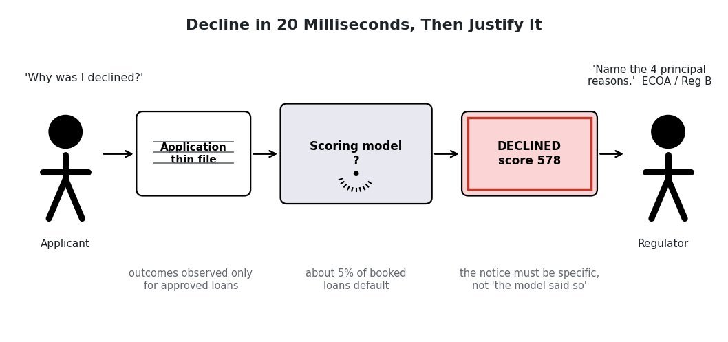
    Line-art scene: an applicant hands a loan application to an opaque scoring machine that returns a DECLINED score, while a regulator on the right demands the four principal reasons

    The Problem: the model can decline an applicant in 20 milliseconds, but the law requires a specific, per-applicant reason, the outcome labels exist only for the people the old model already approved, and any accuracy gain that lands unevenly across groups is a legal liability rather than a win.

    Answer

    The design makes the scoring core explainable by construction instead of bolting an explainer onto a black box. A monotone additive neural network (a neural GAM with one learned shape function per feature) produces the log-odds as a sum of per-feature terms, so each factor’s contribution in score points falls out of the same forward pass that produced the score. A small transaction sequence encoder feeds the additive layer through a handful of named, bounded cash-flow factors, and those few factors are attributed with integrated gradients under a numerically verified completeness check. Two further decisions carry the compliance load: reject inference is solved primarily with a randomized exploration band just below the cutoff plus bureau performance on declined applicants, and fairness is handled by a documented less-discriminatory-alternative search, because group-specific cutoffs would be illegal disparate treatment in consumer credit.

    (1) Explainable-by-Construction Core: a monotone neural GAM over bureau, income, and DTI features, with monotonicity constraints so higher utilization can never lower risk; a GRU over 12 months of transactions contributes 8 named cash-flow factors.
    (2) Exact Attribution Contract: per-feature score-point deltas come from the additive decomposition, integrated gradients cover only the encoder factors, and every explanation is checked against completeness before the notice is issued.
    (3) Reject Inference by Exploration: a randomized approval band on 1% of near-cutoff declines buys unbiased labels below the cutoff; statistical augmentation and bureau outcomes on declines supplement it but never replace it.
    (4) Calibration Over Balance: class weighting during training followed by isotonic recalibration on an unweighted out-of-time holdout, because pricing and expected-loss accounting need a true probability, not a balanced classifier.
    (5) Fairness by Search, Not by Threshold: proxy audits, a less-discriminatory-alternative model search, and adverse impact ratio monitoring with proxy group estimates; the search itself is the compliance artifact.
    (6) One Versioned Artifact: model, monotonicity spec, explainer, and reason-code map ship and are hashed together, so a notice can never be produced by a version that did not make the decision.

    Underwriting pipeline: application to point-in-time feature store to monotone additive scoring core to decision; the attribution engine hangs off the scoring core and feeds the adverse action notice, with a training store and a fairness and drift monitor on the bottom row

    Figure 1: One request produces three artifacts that must agree: a calibrated probability, a decision, and a reason set derived from the same arithmetic that produced the probability.

    Clarify Before Designing:
    (1) Regulatory Scope: US only (ECOA/Reg B plus FCRA adverse action, up to four principal reasons), or also EU GDPR Article 22, which adds a right to human review and changes the automation design?
    (2) Decision Autonomy: is the decline fully automated, or does a human underwriter own a review band where the model is only a recommendation?
    (3) Product and Label Lag: what is the term and the performance definition (90 days past due within 12 months?), since that sets how stale the newest usable training vintage is?
    (4) Volume and Latency: how many applications per day, and is the decision instant at point of sale or allowed to take minutes?
    (5) Reject Data Access: can we pull bureau performance on declined applicants, and does an exploration budget for below-cutoff approvals already exist?
    (6) Protected Attributes: are they collected (mortgage-style) or must disparity be measured with proxy estimates, which changes how much we can trust the fairness numbers?


    Login to view more content
  • MSD0042 Last-Mile Delivery Routing

    Design a deep learning system for last-mile delivery route optimization that predicts travel times, sequences stops, and adapts to real-time traffic and demand. A delivery company such as UPS, FedEx, or Amazon Logistics must route thousands of drivers daily through dense urban and suburban areas, each driver visiting 50-150 stops.

    The system must predict travel times between stops accounting for traffic, time of day, weather, and road type; sequence stops to minimize total time while respecting time windows and vehicle capacity; and re-optimize on the fly when a driver falls behind, a new stop is added, or traffic conditions change. The routing problem is NP-hard at scale, so the system must balance solution quality against compute time, and it must learn from historical route data to improve future predictions.

    How would you design this system? Cover the travel-time prediction model, the route sequencing optimization algorithm (classical VRP solvers vs learned heuristics vs neural combinatorial optimization), the real-time re-optimization strategy, how you incorporate historical route data to improve predictions, and how you evaluate route quality against ground-truth completion times.

    Line-art scene: one delivery van, a scattered cloud of stop markers across a neighborhood, two stops carrying time windows, a new stop appearing mid-shift, a shift clock, and a question mark asking which order

    The Problem: one van, 150 stops, hard time windows, and edge costs that change hour by hour. The number of possible orderings is astronomical, so the system has to guess travel times well and then search the orderings cheaply enough to finish before the shift starts.

    Answer

    The design deliberately splits learning from search. A learned travel-time model turns the road network plus time, weather, and live speed feeds into a time-dependent, distributional cost matrix, and a classical metaheuristic VRP solver (guided local search or hybrid genetic search) sequences the stops against that matrix under time-window and capacity constraints. Deep learning is where it earns its keep, in prediction and in learning driver behavior, not in replacing a solver that must guarantee feasibility. The two pivotal decisions are to predict quantiles rather than mean travel times, so tight windows can be buffered by risk rather than by luck, and to regularize the sequence toward historically executed driver routes, because the Amazon Last Mile Routing Research Challenge showed that cost-optimal sequences are routinely overridden by drivers who know where parking, gates, and one-way alleys actually are. Real-time adaptation is a rolling-horizon re-solve with a frozen prefix, so the plan stays stable in front of the driver while the tail is repaired inside a two-second budget.

    (1) Learned ETA, Classical Search: a road-graph neural network predicts edge travel times; a metaheuristic solver does the combinatorial work with hard feasibility guarantees.
    (2) Distributional Time-Dependent Costs: per-edge p50 and p90 travel times bucketed by departure hour, so rush-hour edges and risky windows are priced correctly.
    (3) Separate Service-Time Model: parking, walking, gates, and elevators are modeled per stop type independently of driving time, because they dominate dense urban routes.
    (4) Driver-Preference Regularization: a zone-sequence model learned from executed routes constrains or penalizes orderings drivers reliably reject.
    (5) Hierarchical Decomposition: sequence delivery zones first, then stops inside each zone, keeping every solver subproblem in the tens of nodes rather than 150.
    (6) Frozen-Prefix Re-optimization: the next few stops are committed; only the tail is re-sequenced by warm-started large neighborhood search under a latency cap.

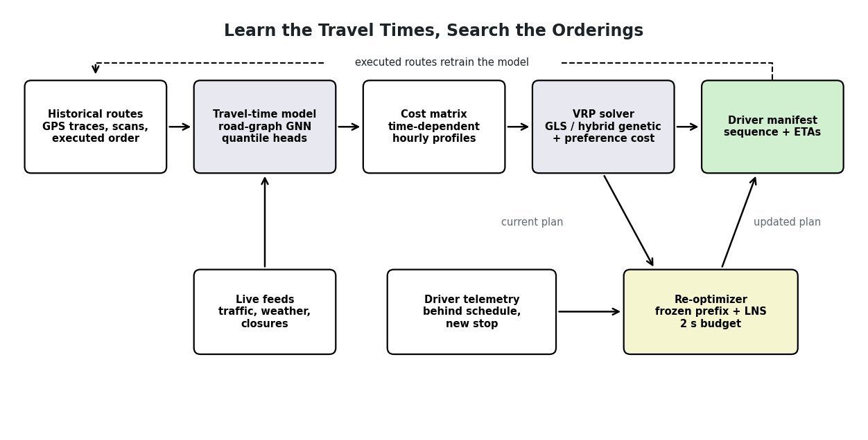
    Routing pipeline: historical routes feed a travel-time model, which builds a time-dependent cost matrix consumed by a VRP solver that emits a driver manifest; live feeds enter the model, driver telemetry triggers a re-optimizer that repairs the plan, and executed routes loop back into training

    Figure 1: Overnight the pipeline runs left to right; during the shift the re-optimizer repairs the tail of an existing plan, and executed routes flow back as training data.

    Clarify Before Designing:
    (1) Scale And Geometry: how many drivers per station per day, how many stops per route, and is the mix dense urban (walking dominated) or suburban (driving dominated)?
    (2) Cost Asymmetry: what does a missed delivery window cost relative to an hour of driver overtime or an extra van dispatched?
    (3) Planning Cadence: is there an overnight batch window with frozen packages, or does volume keep arriving after dispatch?
    (4) Driver Autonomy: must drivers follow the sequence, or may they override, and do we have GPS traces to measure how often they do?
    (5) Label Availability: do we get per-stop arrival and departure timestamps and package scans, or only route start and end times?
    (6) Compute And Connectivity: what solver budget exists per route overnight, what re-optimization latency is acceptable, and can the driver app fall back offline?


    Login to view more content
  • MSD0037 Zillow Personalized Search

    Design Zillow’s “Homes for You” personalized real estate search system that ranks listings by each user’s preferences and browsing behavior. When a user searches for homes in a city, the system must go beyond simple price and size filters to personalize the ranking: a user who repeatedly views Craftsman-style houses with large yards in quiet neighborhoods should see similar listings first, while a first-time searcher gets a diverse, high-quality mix.

    The system must handle cold start for new users, respect hard constraints (price range, location, beds/baths), avoid showing the same listings repeatedly, and balance relevance against inventory freshness, because a listing that went live an hour ago matters more than one that has been sitting for 90 days.

    How would you design this system? Cover the candidate generation and ranking funnel, the user preference signal extraction from browsing behavior, how you handle cold start for new users, the feature set (listing attributes, user history, contextual signals), and the online and offline metrics.

    Line-art scene: a shopper who has browsed many Craftsman homes with big yards looks at a generic ranked feed of condos and townhouses, with notes that the perfect match sits at slot 3 and a two-hour-old listing at slot 48, and a question mark asking which order fits this user

    The Problem: two million active listings, one ranked list, and a shopper whose real preferences (Craftsman, big yard, quiet street) exist only inside their click history. Everyone with the same filters currently sees the same order.

    Answer

    The design is a four-stage funnel: strict hard-constraint filtering, multi-source candidate generation, a learned personalized ranker, and a slate re-ranker that enforces diversity, freshness, and seen-listing decay. Personalization never widens or narrows the legal candidate set. Filters behave like a contract, and learning only reorders what already matches. Two decisions carry the design. First, preferences are extracted as a weighted implicit-feedback profile over listing attributes plus a short in-session view sequence, where a contact-agent event counts far more than a click. Second, cold start is a ramp, not a switch: market-quality priors give way to session signals and then to the full profile as events accumulate. A compliance guardrail sits above everything, because housing personalization is regulated and protected-class proxies cannot be features.

    (1) Hard Filters First: price, beds, baths, geo polygon, and listing status are strict boolean predicates in the search index, so a personalized model can never hide a listing the user explicitly asked for.
    (2) Multi-Source Candidate Generation: union of filter recall (recency-ordered), two-tower ANN retrieval on the user embedding, and co-view/co-save item-item lookups seeded by the session, giving roughly 500 candidates.
    (3) Preference Signal Extraction: event weights (contact 10, save 5, long dwell 2, click 1, hide -3) roll up into a decayed attribute-affinity vector plus the last 20 viewed listing embeddings.
    (4) Learned Ranker: gradient-boosted trees over ~200 listing, user, context, and cross features, trained on a multi-objective label dominated by save and contact events rather than raw clicks.
    (5) Slate Re-Rank: diversity caps per style and block, a bounded new-listing boost, and a seen-decay penalty turn point-wise scores into a slate a human enjoys scrolling.
    (6) Cold Start Ladder and Guardrails: market-quality priors and explore slots for new users, and a feature allow-list plus a neutral-ranker kill switch for Fair Housing compliance.

    Pipeline: search request to hard filters to candidate generation with three sources to ranker to slate re-rank to the Homes for You feed, with an event log feeding a feature store that serves both retrieval and ranking

    Figure 1: The funnel: strict filters define what is legal to show, three retrieval sources decide what is worth scoring, the ranker orders it, and the re-ranker shapes the slate. Behavior events flow back through the feature store into both retrieval and ranking.

    Clarify Before Designing:
    (1) Surface and Scale: is this the in-session search results page, the logged-in “Homes for You” home feed, or the daily email? Each has a different latency budget and a different amount of user history available.
    (2) Filter Semantics: are price and beds hard constraints or soft preferences? If a $520k home may appear for a $500k filter, the whole candidate layer changes.
    (3) Objective: do we optimize saves and agent contacts (monetizable intent) or dwell time? The label choice dictates which behavior the model amplifies.
    (4) Freshness Requirement: what fraction of new listings must receive impressions within 24 hours? This is a marketplace supply guarantee, not a modeling detail.
    (5) Compliance Constraints: which features are off-limits under Fair Housing rules, and does the audit require identical candidate sets for identical filters?
    (6) Data Availability: how much logged-in traffic exists versus anonymous traffic, and can we key profiles on device for anonymous users?


    Login to view more content