Tag: WorldModel

Action-conditioned and generative world models

DL0167 Video Generation Physical Consistency Evaluation

How do you evaluate physical consistency (gravity, collision, object permanence, and temporal coherence) in video and world generation models beyond standard distributional metrics like FID and FVD?

Answer

FID and FVD compare summary statistics of clip embeddings from appearance-biased backbones (InceptionV3, I3D), so they answer whether a set of generated videos resembles a reference set, never whether one clip obeys physics. They are dominated by per-frame content rather than motion, they are nearly insensitive to short-range frame reordering, and they can improve while dynamics get worse. Physical consistency therefore needs per-clip, falsifiable probes. The three that work in practice are: condition the model on the opening frames of a real recorded event and score the predicted continuation against the actual future; ask a calibrated judge (human, or a VLM validated against human labels) for a binary physical-commonsense verdict on each clip; and extract a symbolic readout (track → lift to 3D → fit dynamics) so gravity, momentum, permanence, and flow coherence become numbers with known correct values. For a world model you add a fourth layer, closed-loop rollout, because the only decision-relevant question is whether a policy trained or planned inside the model still succeeds in the real environment.

(1) Distributional vs Per-Clip: FVD is a set-level Frechet distance and cannot label a single video as physically wrong, so it belongs in a regression suite, not in a physics report.
(2) Real-Continuation Probes: give the model the first frames of a genuine recorded event and compare the continuation to ground truth with spatial IoU of the motion mask and masked pixel MSE.
(3) Calibrated Judges: report physical commonsense (PC) and semantic adherence (SA) separately plus their joint pass rate, and publish the judge’s agreement with humans before trusting it.
(4) Symbolic Readout: tracking plus depth lifting turns physics into scalars: fitted gravity residual, momentum error at collisions, occlusion recovery rate, and optical-flow warp error.
(5) Object Permanence Is A Timeline Test: it is only measurable across an occlusion window, so probes must be authored with an occluder and scored on identity, count, and attribute preservation after reappearance.
(6) Closed-Loop For World Models: action-conditioned rollouts are scored by drift over horizon and downstream task success, which is the metric that actually correlates with usefulness.

Diagram of a four-tier evaluation stack: a generated clip with its conditioning fans out to tier one distributional FID and FVD over I3D features, tier two real-continuation probe comparing to a recorded future, tier three calibrated human or VLM judge giving a binary per-clip verdict, and tier four symbolic readout that tracks objects and fits dynamics; each tier emits its own metrics and tiers two to four feed a per-clip physics scorecard while tier one connects with a dashed arrow

Figure 1: The evaluation stack. Only tiers 2 to 4 return a verdict for an individual clip; tier 1 is a distribution-level sanity check whose score can fall (improve) while gravity and collision behaviour degrade, which is exactly why it is drawn with a dashed contribution.

Each of the four physical axes needs a different probe design. Gravity is measured by tracking a free-falling centroid, fitting a quadratic to its height, and comparing the implied acceleration to the reference: generated video overwhelmingly fails toward floaty, slow-motion dynamics with a fitted value well below the true one. Collision is measured at the impact frame, where you check momentum and energy: a coefficient of restitution above 1, interpenetration, or objects passing through each other are hard violations that no appearance metric sees. Object permanence requires a prompt authored with an occluder, then a check that the object reappears with the same identity, count, and colour; the natural scores are the recovery rate and identity-switch count borrowed from multi-object tracking. Temporal coherence is the cheapest to automate: warp consecutive frames with optical flow, mask out occlusions and disocclusions, and average the residual, which catches flicker, texture swimming, and morphing that a per-frame FID is blind to. Crucially, all four scores are reported as per-clip pass rates over a curated probe set, not as an average of a continuous score, because averaging hides the fact that most failures are categorical.

Mathematical Formulation:
$d_F^2 = \| \mu_r - \mu_g \|_2^2 + T_{\Sigma}$
$T_{\Sigma} = \mathrm{Tr}(\Sigma_r + \Sigma_g - 2 (\Sigma_r \Sigma_g)^{1/2})$
$y(t) = y_0 + v_0 t + \frac{1}{2} \hat{g} t^2$
$e_g = | \hat{g} - g | / g$
$e_p = \| p^{+} - p^{-} \| / \| p^{-} \|$
$R_p = N_{\mathrm{rec}} / N_{\mathrm{occ}}$
$\tilde{I}_t = \mathcal{W}(I_t, f_{t \to t+1})$
$\epsilon_t = \| m_t \odot (I_{t+1} - \tilde{I}_t) \|_1$
$E_w = \frac{1}{T-1} \sum_{t=1}^{T-1} \epsilon_t$
$J = \frac{1}{N} \sum_{i=1}^{N} c_i^{\mathrm{pc}} c_i^{\mathrm{sa}}$

Where:

$d_F^2$ is the FVD value, with $\mu_r, \Sigma_r$ and $\mu_g, \Sigma_g$ the mean and covariance of real and generated clip features from a fixed video backbone; it is defined only over sets, which is the root of its uselessness for per-clip physics.
$y(t)$ is the tracked height of an object at time $t$ , $y_0$ and $v_0$ the fitted initial height and velocity, and $\hat{g}$ the least-squares acceleration recovered from the generated clip; $e_g$ is its relative error against the reference $g$ .
$p^{-}$ and $p^{+}$ are total momentum immediately before and after a contact frame, so $e_p$ is the relative momentum violation; the same construction on kinetic energy exposes a restitution above 1.
$N_{\mathrm{occ}}$ is the number of authored occlusion events and $N_{\mathrm{rec}}$ the number where the object reappears with correct identity, count, and attributes, giving the permanence recovery rate $R_p$ .
$\mathcal{W}$ is backward warping by the estimated flow $f_{t \to t+1}$ , $m_t$ the binary validity mask that removes occluded and out-of-frame pixels, $\odot$ elementwise product, and $E_w$ the averaged warp error over the $T$ frames.
$c_i^{\mathrm{pc}}, c_i^{\mathrm{sa}} \in \{0,1\}$ are the physical-commonsense and semantic-adherence verdicts on clip $i$ , so $J$ is the joint pass rate: a clip counts only if it is both on-prompt and physically plausible.

Two-panel chart. Left panel plots tracked height versus time for a reference bouncing ball following ballistic arcs with decaying apex heights and a generated clip that falls more slowly, dips below the floor line, and rebounds to an apex higher than its release height. Right panel plots speed magnitude versus time, showing the reference speed dropping from about 9.9 to 7.4 metres per second at impact while the generated clip's speed increases from about 6.6 to 7.6 metres per second at impact

Figure 2: The symbolic readout on one probe clip. The fitted acceleration is 4.2 instead of 9.8, the object interpenetrates the floor, and the post-impact speed exceeds the pre-impact speed (restitution above 1, so energy is created). Every one of these is a numeric, falsifiable failure; all of them are invisible to a distributional metric computed on the same clip.

Metric family	Granularity	What it catches	What it misses
FID / FVD	Set level, needs hundreds of clips	Gross artefacts, blur, mode collapse, distribution shift	All per-clip physics; content bias makes it track texture more than motion
Real-continuation probe	Per clip, against recorded ground truth	Wrong outcome of a near-deterministic event (where a ball lands, whether paint mixes)	Legitimate stochastic futures are penalised unless you score a sampled set
Calibrated human or VLM judge	Per clip, binary PC and SA	Open-ended violations on arbitrary prompts, including material and state-change errors	Sub-second and geometric violations; judge agreement with humans is far from perfect
Symbolic trajectory readout	Per clip, per object, per frame	Gravity residual, momentum and energy errors, interpenetration, identity switches, warp error	Anything the tracker or depth model cannot follow: fluids, smoke, cloth, heavy occlusion
Closed-loop rollout	Per episode, action-conditioned	Compounding drift and any error that actually changes a policy’s decision	Expensive, needs an action-conditioned model plus a real or simulated environment

August 19, 2026

DL0166 3D Gaussian and NeRF Neural Simulator

How do 3D Gaussians and Neural Radiance Fields serve as dense physical representations inside differentiable neural simulators?

Answer

A differentiable neural simulator needs one scene description that works twice: as geometry the solver can push around, and as an image the photometric loss can compare against real video. NeRF supplies the second half well, storing the scene as an implicit field that maps a position and view direction to density and radiance, rendered by differentiable volume quadrature along rays. What it lacks is handles, because an MLP field has no particle to give mass, no covariance to advect, and no obvious place to attach a constitutive model. 3D Gaussian Splatting removes that obstacle by storing the scene as an explicit set of anisotropic Gaussians with mean, covariance, opacity, and spherical-harmonic color, so every primitive doubles as a material point in a Lagrangian solver. The simulator advances those points with differentiable physics, usually MLS-MPM, the rasterizer splats them back to pixels, and gradients from the rendering loss flow through both the rollout and the renderer into material parameters such as Young’s modulus, Poisson ratio, yield stress, and friction. The loop is therefore video → physical parameters → rollout of unseen dynamics, with pixels as the only supervision.

(1) Dense Means Physics Everywhere: unlike a mesh, both representations describe the interior volume, so mass, velocity, and stress are defined at every sampled point rather than only on a surface shell.
(2) Gaussians Are Already Particles: a splat’s mean is a particle position and its covariance is a local volume element, which is exactly the state an MPM particle carries, so the reconstruction and the simulation share one data structure.
(3) NeRF Needs A Bridge: a continuous field has to be voxelized or resampled onto particles each step, the Eulerian-Lagrangian conversion that PAC-NeRF introduced, which costs an extra transfer and an extra source of gradient noise.
(4) Covariance Follows The Deformation Gradient: kinematics are preserved by advecting the mean through the flow map and conjugating the covariance with $F$ , otherwise stretched material still renders as undeformed blobs.
(5) The Loss Is Purely Photometric: no ground-truth stiffness is available, so system identification is driven by rendered-versus-observed pixel error over a multi-frame rollout.
(6) The Cost Lives In The Backward Pass: memory grows as $O(TN)$ in substeps and particles, and gradients through contact and friction are non-smooth, so checkpointing and softened contact models are mandatory.

Left-to-right pipeline: multi-view video with camera poses feeds a dense reconstruction stage producing 3D Gaussians or a NeRF field, which becomes a physical particle state with mass, velocity and deformation gradient, advanced by a differentiable MPM simulator, rendered by a differentiable renderer and compared to the observed frames, with a dashed backward gradient path into a material parameter block that feeds the simulator

Figure 1: The identification loop. The dense representation appears twice in the graph, once as the initial physical state and once as the thing being rendered, which is why gradients from a single photometric loss can reach material parameters that were never observed directly.

The reason 3D Gaussians displaced radiance fields in this role is mechanical rather than aesthetic. In a Lagrangian solver the unknowns are particle positions and their local deformation, and a Gaussian already stores a mean plus a covariance factored as scale and rotation, so PhysGaussian can drive splats directly with a continuum solver and keep rendering in real time. A radiance field, by contrast, is a function of space with no identity attached to any location, so tracking material requires either a learned deformation field mapping observation time back to a canonical frame, or a particle proxy that carries the physics while the field carries appearance. Two consequences matter in practice. First, the spherical-harmonic coefficients are expressed in world coordinates, so when a splat rotates by $R$ its appearance basis must be rotated too, otherwise highlights stay welded to the world frame while the geometry turns. Second, lighting is baked, so shadows and specular reflections do not respond to motion, which biases the photometric gradient exactly on the frames where an object moves most.

Two panels of ellipse grids: the left panel shows a three by three grid of identical circular Gaussians in the rest state, the right panel shows the same grid after a shear and vertical compression, where each ellipse is stretched and tilted consistently with the displaced particle centers, connected by an arrow labelled F

Figure 2: Kinematics of a splat. The mean rides the flow map while the covariance is conjugated by the deformation gradient, so shear and compression change both where a Gaussian sits and how it is shaped; skipping the covariance update leaves visibly isotropic blobs inside sheared material and corrupts the rendering gradient.

Mathematical Formulation:
$\alpha_i = 1 - \exp(-\sigma_i \delta_i)$
$T_i = \prod_{j=1}^{i-1}(1 - \alpha_j)$
$C(r) = \sum_{i=1}^{N} T_i \alpha_i c_i$
$\Sigma = R S S^\top R^\top$
$\mu_p^{t} = \phi_t(\mu_p^{0})$
$\Sigma_p^{t} = F_p^{t}\,\Sigma_p^{0}\,(F_p^{t})^\top$
$s_{t+1} = \mathcal{S}(s_t;\theta)$
$\mathcal{L} = \sum_t \lVert \mathcal{R}(s_t) - I_t \rVert^2$
$\nabla_{\theta}\mathcal{L} = \sum_t \frac{\partial \mathcal{L}}{\partial s_t}\frac{\partial s_t}{\partial \theta}$

Where:

$C(r)$ is the rendered color of ray $r$ , accumulated over $N$ ordered samples or splats with per-sample color $c_i$ ; this same alpha-compositing form covers NeRF quadrature and Gaussian splatting.
$\sigma_i$ is density, $\delta_i$ the sample spacing along the ray, $\alpha_i$ the resulting opacity, and $T_i$ the transmittance reaching sample $i$ .
$\Sigma$ is a splat’s covariance, parameterized by rotation $R$ and diagonal scale $S$ so that it stays positive semi-definite under gradient updates.
$p$ indexes particles, $\phi_t$ is the flow map from rest to time $t$ , and $F_p^{t} = \partial \phi_t / \partial \mu$ is the deformation gradient whose determinant gives local volume change.
$s_t$ is the full simulator state (positions, velocities, $F$ , affine momentum) and $\mathcal{S}$ one differentiable substep.
$\theta$ collects the unknown physical parameters such as Young’s modulus $E$ , Poisson ratio $\nu$ , density $\rho$ , yield stress, and friction coefficient.
$\mathcal{R}$ is the differentiable renderer and $I_t$ the observed frame, so $\mathcal{L}$ is a multi-frame photometric residual and its gradient is a product of per-substep Jacobians.

That last product is where the engineering happens. Explicit MPM needs a CFL-limited timestep, so one video frame at 30 fps typically hides a few hundred substeps, and reverse-mode differentiation over a one-second clip means backpropagating through several thousand Jacobians. Storing every intermediate state is what kills the run: 200k particles at roughly 96 bytes of state per particle is about 19 MB per substep, so a 1,000-substep rollout needs 19 GB of tape. The standard remedies are gradient checkpointing at an interval near $\sqrt{T}$ , truncating the loss window to a handful of frames, and recomputing forward segments during the backward pass. Numerically, the same product of Jacobians makes gradients explode for stiff materials and vanish once the trajectory has been dissipated by friction, which is why practitioners fit a log-parameterized stiffness and soften contact before trusting any gradient at all.

Log-log chart of backward-pass memory in bytes versus number of simulator substeps for 200 thousand particles, comparing storing the full trajectory which grows linearly and reaches 40 gigabytes near 2000 substeps, against square-root gradient checkpointing which stays under 3 gigabytes, with a dash-dotted horizontal line marking a 40 gigabyte HBM budget

Figure 3: Why differentiable rollouts are short. At 19 MB of particle state per substep, the naive tape exhausts a 40 GB HBM budget after roughly 2,000 substeps, about one second of simulated time, while square-root checkpointing keeps memory in the low gigabytes at the price of one extra forward pass.

Property	NeRF (implicit field)	3D Gaussians (explicit primitives)
Primitive	MLP or hash grid queried at continuous positions; no persistent identity	Set of anisotropic Gaussians, each with mean, covariance, opacity, SH color
Coupling to solver	Needs a deformation field or an Eulerian-Lagrangian resampling step onto particles	Splat is used directly as an MPM material point, no conversion layer
Render cost per frame	Hundreds of network queries per ray; typically tens of ms to seconds	Tile-based rasterization, real time at 1080p on one GPU
Handles topology change	Naturally, since density is just a field value that can appear or vanish	Poorly; fracture needs splitting or spawning new Gaussians outside the solver
Dominant failure mode	Slow rollouts, floaters in unobserved regions, noisy gradients through resampling	Baked lighting and unrotated SH, plus spiky splats that behave like bad particles

August 19, 2026

DL0165 End-to-End Driving Trajectory Scoring

How do end-to-end autonomous driving architectures combine world model generation with trajectory scoring and cost function evaluation to select the safest driving path?

Answer

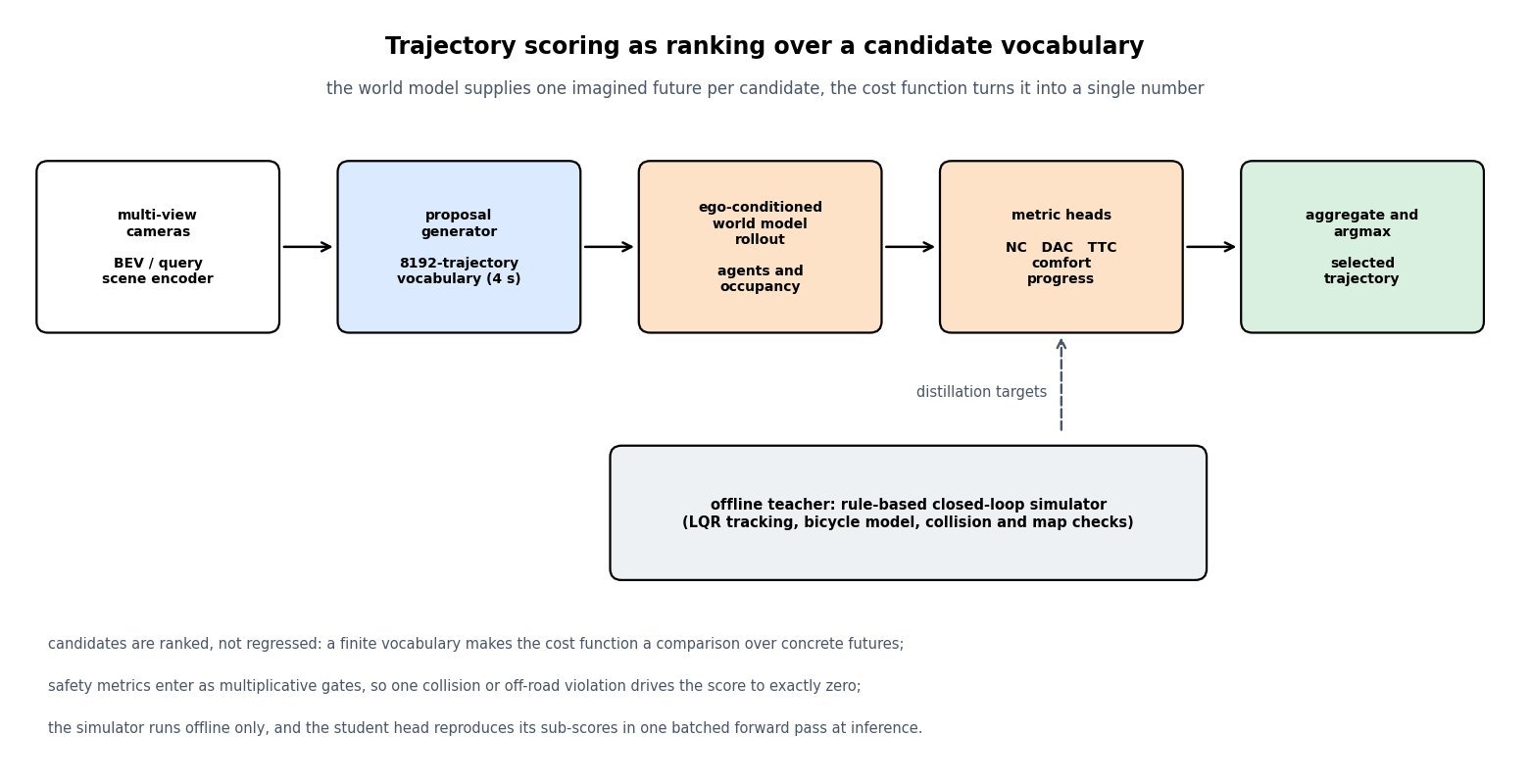
Competitive end-to-end stacks do not regress one trajectory and drive it. They propose many candidates, imagine the future under each one, and then take the argmax of an explicit cost, which turns planning into a ranking problem over a finite action set. The world model is what makes the ranking meaningful: it is an ego-conditioned forecaster that answers a counterfactual question, namely what the agents, the occupancy grid, or the camera views would look like if this particular trajectory were executed. The cost function then reads that imagined rollout and produces bounded sub-metrics for collision, drivable-area compliance, time-to-collision, comfort, and progress, which are combined so that hard safety terms multiply and soft preference terms are averaged. Because rolling out a simulator for thousands of candidates is far too slow at a 10 Hz replanning rate, production designs run the expensive scorer offline as a teacher and distill it into a small scoring head that evaluates the whole vocabulary in one batched forward pass.

(1) Proposal Set Instead Of Regression: a fixed trajectory vocabulary (8192 clustered 4-second trajectories in Hydra-MDP, 4096 in VADv2) or a small set of diffusion anchors preserves multi-modality and gives the cost function something concrete to compare.
(2) Ego-Conditioned World Model: the rollout must be conditioned on the candidate action, otherwise every candidate shares one predicted future and the scores carry no causal information about the ego’s own choice.
(3) Multiplicative Gates Plus Weighted Soft Terms: collision and off-road terms enter as multiplicative factors so a single violation zeroes the score, while time-to-collision, comfort, and progress enter as a weighted average that only re-ranks the survivors.
(4) Simulator As Teacher, Head As Student: a rule-based closed-loop metric computed with LQR tracking on a bicycle model labels every candidate offline, and a cross-attention scoring head learns those labels, converting a multi-second simulation into a millisecond-scale inference.
(5) Reactivity Decides Validity: non-reactive rollouts hold other agents on their logged paths, which systematically over-rewards cutting in and under-penalizes aggressive gap acceptance.
(6) Latency Sets The Design: a 4-second horizon at 10 Hz is 40 poses per candidate and the whole loop must close inside about 100 ms, which rules out per-candidate video generation online.

Left-to-right pipeline diagram: multi-view camera BEV scene encoder, then a proposal generator producing a vocabulary of 8192 four-second trajectories, then an ego-conditioned world model rollout predicting agent futures and occupancy for each candidate, then metric heads for no at-fault collision, drivable area compliance, time-to-collision, comfort and progress, then score aggregation and argmax selecting one trajectory, with an offline rule-based simulator below feeding distillation targets into the metric heads

Figure 1: One scene encoder, many candidates, one score. The world model rollout is evaluated per candidate, and the metric heads are trained against an offline rule-based simulator, so the simulator’s judgement is available at inference without running it.

The world model shows up in three distinct roles, and confusing them is a common interview mistake. In the in-loop role, a generative model such as Drive-WM synthesizes multi-view future frames conditioned on each candidate and an image-space reward built from map and object cues picks the branch, which is expressive but so expensive that only a shallow tree of a few branches is affordable. In the representation role, future-occupancy or future-agent forecasting is an auxiliary head that shapes the BEV latent, so cost terms are computed on predicted geometry rather than pixels, which is the practical choice inside a 100 ms budget. In the offline role, high-fidelity generators supply rare scenarios and closed-loop training environments, so the cost function is validated against near-misses that almost never appear in logged data. Whatever the role, the failure mode is the same: if the rollout ignores that other agents respond to the ego, the cost function rewards trajectories that would have been vetoed by any reactive simulator.

Bird's-eye-view schematic of a two-lane road with an ego vehicle, a slow lead vehicle ahead in the same lane, and a vehicle in the left lane. Four candidate trajectories are drawn: an overtake into the left lane that collides with the left-lane vehicle and scores zero, a swerve onto the non-drivable shoulder that also scores zero, a full-stop brake that stays legal but has near-zero progress and scores 0.48, and a lane-keeping follow trajectory that scores 0.92 and is selected

Figure 2: Why the aggregation is multiplicative rather than additive. Candidates A and B are gated to exactly zero by collision and drivable-area violations no matter how much progress they buy, and only then do the soft terms separate the timid full stop from the trajectory that actually makes progress.

Mathematical Formulation:
$\hat{s}_{t+1:t+H} \sim p_{\phi}(\cdot \mid o_{\leq t}, \tau)$
$f_m(\tau) = g_m(\hat{s}_{t+1:t+H})$
$P(\tau) = \prod_{m \in \mathcal{M}_g} f_m(\tau)$
$Q(\tau) = \frac{\sum_m w_m f_m(\tau)}{\sum_m w_m}$
$S(\tau) = P(\tau) \cdot Q(\tau)$
$\tau^{*} = \arg\max_{\tau \in \mathcal{V}} S(\tau)$

Where:

$\tau^{*}$ is the executed trajectory and $\mathcal{V}$ the candidate vocabulary, typically a few thousand clustered 4-second trajectories sampled at 10 Hz.
$o_{\leq t}$ is the sensor history, $p_{\phi}$ the ego-conditioned world model, and $\hat{s}_{t+1:t+H}$ the imagined future over horizon $H$ under that specific $\tau$ .
$g_m$ extracts metric $m$ from the rollout and $f_m(\tau)$ is its value, bounded to the unit interval so that scores are comparable across scenes.
$\mathcal{M}_g$ are the gate metrics (no at-fault collision, drivable-area compliance) whose product $P(\tau)$ vetoes a candidate outright.
$w_m$ are the weights of the soft metrics (time-to-collision, comfort, ego progress) aggregated by $Q(\tau)$ , which only re-ranks candidates that passed every gate.

NAVSIM PDM Score Instantiation:
$S = \mathrm{NC} \cdot \mathrm{DAC} \cdot Q$
$Q = (5\,\mathrm{TTC} + 2\,\mathrm{C} + 5\,\mathrm{EP}) / 12$

Here NC and DAC are binary gates, while time-to-collision, comfort, and ego progress carry weights 5, 2, and 5. The weights are the policy: raising the progress weight produces a stack that squeezes through gaps, and raising comfort produces one that refuses to brake late. The distillation objective simply asks the student head to reproduce every teacher sub-metric per candidate.

Distillation And Latency Budget:
$\mathcal{L} = \sum_{\tau} \sum_m \mathrm{BCE}(\hat{f}_m(\tau), f_m^{\mathrm{sim}})$
$t_{perc} + t_{gen} + t_{score} \leq 100\ \mathrm{ms}$
$40\ \mathrm{ms} + 25\ \mathrm{ms} + 15\ \mathrm{ms} = 80\ \mathrm{ms}$

Log-log chart of scoring latency in milliseconds against the number of scored candidate trajectories, with three curves: a distilled learned scoring head that stays nearly flat from 14 to about 32 milliseconds up to 8192 candidates, a rule-based closed-loop simulator that grows linearly at roughly 0.45 milliseconds per candidate, and a generative video world model rollout at roughly 320 milliseconds per candidate, plus a dashed horizontal line marking a 100 millisecond replanning budget

Figure 3: Representative per-candidate costs against the 100 ms replanning budget. A distilled scoring head is almost flat in the number of candidates because scoring is one batched forward pass, a rule-based simulator caps out near a hundred candidates, and a per-candidate video rollout blows the budget on its first branch.

Property	Rule-based simulator in the loop	Generative world model in the loop	Distilled learned scorer
Proposal source	Centerline offsets crossed with target speeds, about 15 proposals	A shallow tree of a few branches per replan	Clustered vocabulary of 4096 to 8192 trajectories, or 20 diffusion anchors
How futures are obtained	Bicycle model plus LQR tracking with map and collision checks	Diffusion rollout of multi-view frames or occupancy conditioned on the action	No explicit rollout at inference, the head predicts each sub-metric directly
Agent reactivity	Configurable, IDM background traffic reacts to the ego	Learned and implicit, quality depends entirely on training data	Inherited from whatever the teacher assumed, usually non-reactive logs
Per-candidate cost	Sub-millisecond but CPU-bound and linear in candidates	Hundreds of milliseconds of GPU time per branch	Microseconds, batched inside one transformer forward pass
Dominant failure mode	Hand-written dynamics and a coarse proposal set miss creative maneuvers	Hallucinated geometry, action leakage, and unusable latency	Copies the teacher’s blind spots and can latch onto ego-status shortcuts

August 19, 2026

DL0164 BEV Transformation: Lift-Splat-Shoot

Explain Bird’s-Eye-View transformation methods such as Lift-Splat-Shoot and transformer cross-attention for mapping multi-view camera video into a unified 3D world representation, as used in camera-only autonomous driving stacks and benchmarked on nuScenes.

Answer

A BEV transformation converts $N_{c}$ perspective images, each of which has thrown away the depth of every pixel, into a single metric grid in the ego frame where one cell always means the same physical patch of ground. Every method must invent the missing depth, and the two families differ only in which direction they move information. Forward projection, introduced by Lift-Splat-Shoot (LSS), predicts a categorical depth distribution per pixel, lifts each pixel into a frustum of $D$ candidate 3D points weighted by that distribution, then splats the points into BEV pillars with sum pooling. Backward projection, popularised by BEVFormer, starts from a fixed set of learned BEV queries, projects each query’s 3D anchor points into every camera using the known intrinsics and extrinsics, and pulls features back with deformable cross-attention so no explicit depth prediction is required. Both produce the identical output contract, typically a $200 \times 200 \times 256$ feature map at roughly 0.5 m resolution, which is why detection, map segmentation, occupancy and planning heads can be shared, and both add temporal fusion by warping the previous BEV feature into the current ego frame before merging.

(1) The Core Difficulty Is Depth, Not Geometry: the pixel-to-ray mapping $K^{-1}$ and the camera-to-ego rigid transform are exactly known, so the only unknown is the scalar range along each ray.
(2) Forward Projection (Push): LSS predicts $\alpha_{u,v,d}$ over $D$ discrete depth bins, takes an outer product with the context feature, and voxel-pools the resulting frustum point cloud into pillars.
(3) Backward Projection (Pull): BEV queries carry their own 3D position, project into the cameras that actually see them, and sample features with deformable attention, which sidesteps depth estimation entirely.
(4) Shared Output Contract: both write into the same ego-frame grid, so the transformation is a swappable module rather than an architecture commitment.
(5) Temporal Recurrence Is Not Optional: warping $B_{t-1}$ by the ego pose delta and fusing it into $B_{t}$ is what makes velocity estimation and short-occlusion memory possible from cameras alone.
(6) Depth Supervision Decides Accuracy: BEVDepth showed that supervising $\alpha$ with LiDAR-projected depth, rather than letting the detection loss shape it, is the single largest quality lever for the forward family.

Pipeline diagram: six surround cameras feed a shared 2D backbone with FPN, which splits into a top lane predicting a per-pixel depth distribution over 59 bins followed by an outer product and voxel pooling of roughly one million frustum points, and a bottom lane of learned 200 by 200 BEV queries whose 3D anchors are projected into the hit cameras for deformable cross-attention over image features used as keys and values; both lanes write into one 200 by 200 by 256 unified BEV feature map that feeds detection, map and occupancy heads

Figure 1: Two directions, one destination. The push lane commits to a depth distribution and scatters features outward; the pull lane keeps the grid fixed and gathers features inward. Everything downstream of the unified BEV feature map is identical, which is why these modules are interchangeable in practice.

The forward path is best understood as a soft, differentiable version of unprojecting a depth map. A pixel with context feature $c_{u,v} \in \mathbb{R}^{C}$ does not pick one depth; it spreads that feature over all $D$ bins in proportion to $\alpha_{u,v,d}$ , so a confident pixel deposits nearly all of its mass in one pillar while an ambiguous pixel smears a faint trail along its ray. Because the splat is a sum, the operation is permutation-invariant and handles overlapping camera fields of view for free, and because it is differentiable, gradients reach the depth head through the pooling. The engineering cost is the frustum point count, which is why production implementations replace the naive scatter with a sorted cumulative-sum pooling kernel or a preallocated BEVPoolv2 index table that skips materialising the point cloud at all.

Three panels: a grid of image pixels with one highlighted pixel carrying a 256-dimensional context feature; a bar chart of the predicted probability over 59 depth bins showing a sharp peak near 18 metres for a confident pixel and a broad dashed curve for an ambiguous pixel; and a top-down bird's-eye-view grid with the camera at the origin, a ray fanning outward, circles along the ray whose size is proportional to the depth probability, and one highlighted 3 by 3 metre pillar where the points are sum-pooled

Figure 2: One pixel becomes $D$ weighted 3D points. The width of the depth distribution is literally the width of the smear in BEV, so a flat $\alpha$ over a textureless road or a night-time scene produces a long low-confidence streak instead of a localised object.

Forward Projection (Lift-Splat-Shoot):
$\tilde{u} = (u, v, 1)^{T}$
$p_{c} = d\, K^{-1} \tilde{u}$
$p_{e} = R\, p_{c} + t$
$F_{u,v,d} = \alpha_{u,v,d}\, c_{u,v}$
$\sum_{d=1}^{D} \alpha_{u,v,d} = 1$
$B(x,y) = \sum_{p \in \Pi(x,y)} F(p)$

Where:

$B(x,y) \in \mathbb{R}^{C}$ is the BEV feature at grid cell $(x,y)$ in the ego frame, and $\Pi(x,y)$ is the set of frustum points whose ego coordinates fall inside that pillar.
$\tilde{u}$ is the homogeneous pixel coordinate, $K$ the camera intrinsic matrix, and $(R, t)$ the camera-to-ego extrinsic rotation and translation.
$d$ indexes the depth bins, with $d \in \{1, \ldots, D\}$ over a fixed range such as 1 m to 60 m in 1 m steps, giving $D = 59$ .
$\alpha_{u,v,d}$ is the softmax depth distribution for pixel $(u,v)$ and $c_{u,v}$ its context feature, so $F_{u,v,d}$ is the outer-product lift.
The splat is sum pooling, which keeps the operation order-free across cameras and differentiable with respect to both $\alpha$ and $c$ .

The backward path inverts the flow of information. A query at grid cell $(x,y)$ is lifted to $N_{z}$ anchor heights along a vertical pillar, each anchor is projected into every camera, and only the cameras whose image plane actually contains the projection contribute. Deformable attention then samples a handful of learned offsets around each projected location, so cost scales with the number of queries rather than with image resolution times depth bins, and a query near a lane boundary can shift its sampling points to where the evidence is instead of trusting a predicted depth. The trade-off is that the geometry is now an attention prior rather than a hard constraint: if extrinsics are wrong, the network can still learn to compensate, which is convenient during training and dangerous during deployment because the failure is silent.

Backward Projection (Cross-Attention):
$q_{xy} = Q(x,y) + \mathrm{PE}(x,y)$
$r_{j} = (x, y, z_{j})$
$\hat{p}_{ij} = \pi_{i}(r_{j})$
$A_{i} = \sum_{j=1}^{N_{z}} \mathrm{DA}(q_{xy}, \hat{p}_{ij}, F_{i})$
$\mathrm{CA}(q_{xy}) = \frac{1}{|V_{xy}|} \sum_{i \in V_{xy}} A_{i}$

Where:

$\mathrm{CA}(q_{xy})$ is the cross-attention output written into BEV cell $(x,y)$ , and $q_{xy}$ is the learned query plus its 2D positional encoding.
$r_{j}$ is the $j$ -th pillar anchor at height $z_{j}$ , with $N_{z} = 4$ a common choice spanning roughly -5 m to 3 m.
$\pi_{i}$ is the full projection of camera $i$ , so $\hat{p}_{ij}$ is a sub-pixel image location and $F_{i}$ the multi-scale feature map of that camera.
$V_{xy}$ is the set of cameras whose frustum contains at least one anchor, so the average is taken only over hit views and empty views contribute nothing.
$\mathrm{DA}$ is deformable attention, which samples a few learned offsets around $\hat{p}_{ij}$ with bilinear interpolation instead of attending to all pixels.

Frustum Cost At A Typical Configuration:
$N_{pts} = N_{c} \cdot H \cdot W \cdot D$
$6 \times 32 \times 88 \times 59 = 996864$
$200 \times 200 = 40000$

Roughly one million frustum points collapse into forty thousand pillars, an average of about 25 points per cell, and that ratio is exactly why the pooling kernel rather than the backbone is often the latency bottleneck in the forward family. It also exposes the accuracy story: because every point sits on a known ray, a lateral mistake of one pixel at 50 m is only about 4 cm, while a 5% depth mistake at the same range is 2.5 m. BEV error is dominated by range error, and it grows linearly with distance.

Log-scale line chart of bird's-eye-view position error in metres against range from the ego vehicle from 2 to 80 metres, showing straight rising lines for 10 percent, 5 percent and 2 percent relative depth error, and a much lower line for a one-pixel lateral error at focal length 1266 pixels, with a dashed horizontal line at the 2 metre matching threshold and an annotation noting that a 5 percent depth error at 60 metres displaces the box by 3 metres

Figure 3: Range error, not image-plane error, sets BEV quality. A one-pixel lateral error stays under 10 cm across the whole working range, while a modest relative depth error crosses the 2 m matching threshold somewhere between 20 m and 100 m depending on the depth head, which is why depth supervision and long-baseline temporal stereo pay off so heavily.

Property	Forward push (LSS, BEVDet, BEVDepth)	Backward pull (BEVFormer)	Implicit 3D encoding (PETR)
Depth handling	Explicit categorical distribution over D bins, optionally LiDAR-supervised	No depth head; anchors at fixed pillar heights sample every hit view	3D coordinates baked into image position encodings, depth learned implicitly
Dominant cost	Frustum scatter of about 1M points; needs a cumsum or index-table kernel	40,000 queries times layers times sampling points, quadratic in grid side	Global attention over all image tokens, no explicit BEV grid to build
Calibration sensitivity	Hard geometric constraint, so extrinsic drift shifts features into wrong pillars	Attention can partly absorb drift, which hides the fault instead of surfacing it	Most tolerant, but least interpretable when a single camera goes bad
Temporal fusion	Warp and concatenate past BEV grids, or run temporal stereo across frames	Recurrent BEV self-attention on the ego-warped previous grid	Propagate sparse object queries forward in time, no grid to warp
Typical failure	Flat depth distribution smears a distant object along its ray	Empty cells still consume compute, and unseen regions hallucinate from priors	Weak spatial locality makes small distant objects easy to miss

August 19, 2026

DL0163 Map-Based vs Mapless World Models

How do map-based world models conditioned on HD-maps differ from end-to-end mapless world models that predict from raw sensor observations, for a driving stack like Waymo’s or Wayve’s?

Answer

Both families learn a latent transition model that rolls the scene forward under a candidate ego action, so the architectural difference is not the dynamics head but what the dynamics head is allowed to condition on. A map-based world model receives a local HD-map crop $m_t$ , a rasterized or vectorized patch of lane centerlines, stop lines, crosswalks, and traffic-light-to-lane associations, indexed out of a global map by the pose that the localization stack estimates. That crop enters as a hard geometric prior, so the network never has to learn road topology from pixels and can spend capacity on agent behavior. A mapless model sees only the sensor history $o_{t-k:t}$ and must reconstruct that same topology inside its latent on every frame, which is statistically much harder but works on roads nobody has surveyed. The practical result is a swap of error sources rather than a strict improvement: the map-based system inherits map staleness and localization error, the mapless system inherits data hunger and weaker long-horizon geometric consistency.

(1) Conditioning Set: map-based factorizes as $p(z_{t+1} \mid z_t, a_t, m_t)$ with an extra exogenous input, while mapless factorizes as $p(z_{t+1} \mid z_{t-k:t}, a_t)$ and must carry topology in the recurrent state.
(2) Where The Prior Lives: in one system lane geometry is a surveyed asset refreshed by a mapping fleet, in the other it is weights learned from driving video.
(3) Sample Efficiency: handing the model the road graph removes an enormous nuisance factor, so map-conditioned models converge on thousands of hours where mapless generative models are trained on tens of thousands to millions.
(4) Failure Signature: a stale or misaligned map produces confidently wrong rollouts, whereas a mapless model facing an ambiguous road typically produces a wide, visibly uncertain distribution.
(5) Pose Coupling: the map crop is only meaningful in the correct frame, so map-based prediction quality is bounded by localization accuracy; mapless prediction has no pose dependency at all.
(6) Scaling And ODD: map-based scales with surveyed kilometers and re-survey cadence, mapless scales with data and compute, which is why geofenced robotaxi and everywhere-consumer programs made opposite choices.

Two stacked pipelines: the upper map-based pipeline encodes surround camera and LiDAR into a latent state, takes an HD map crop selected by ego pose as an extra conditioning input to the transition model, and decodes BEV occupancy, agent futures, and an ego plan; the lower mapless pipeline tokenizes surround camera video, feeds a spatio-temporal transformer or diffusion prior conditioned only on past tokens and the action, and decodes future frames, an implicit map, and an ego plan

Figure 1: The two stacks share an encoder, a latent transition model, and a decoder. Only one extra edge differs: the HD map crop selected by the estimated pose feeding the transition model. That single edge is what buys sample efficiency and what imports two new failure sources, map staleness and localization drift.

The interesting behavior appears when the map and the world disagree. Because the map is treated as ground truth during training, the model learns to trust it, and at inference it has no mechanism to discount it: a lane that was closed for construction last week is still a valid lane inside $m_t$ , so the imagined rollout drives straight through the closure with low predictive variance. A mapless model never had that crutch, so its estimate of drivable space comes from the same pixels that show the cones. It pays for this with weaker long-horizon geometry, since nothing anchors an eight-second rollout to a globally consistent lane graph and errors compound in the latent. This is also why the honest comparison is not accuracy on a nominal benchmark, where the map-conditioned model almost always wins, but accuracy conditioned on map validity.

Two bird's-eye-view panels of the same two-lane road with a lane closure marked by cones. In the left map-based panel a blue HD map centerline runs straight through the closure and the predicted rollout follows it with a narrow uncertainty band, ending in a red cross at the cones. In the right mapless panel there is no map centerline, the predicted rollout bends into the adjacent lane around the cones, and the uncertainty band is visibly wider.

Figure 2: Same scene, same closure, different conditioning. The map prior keeps the rollout tight and correct whenever the map matches reality, and keeps it tight and wrong when it does not. The mapless rollout is wider but reactive, because the only evidence it ever had for drivable space is the current image.

Mathematical Formulation:
$z_t = E_\theta(o_{t-k:t})$
$m_t = \Pi(M, \hat{T}_t), \quad \hat{T}_t = T_t + \epsilon_{\mathrm{loc}}$
$p_{\mathrm{map}} = p_\theta(z_{t+1} \mid z_t, a_t, m_t)$
$p_{\mathrm{free}} = p_\phi(z_{t+1} \mid z_{t-k:t}, a_t)$
$\mathcal{L} = \sum_{h=1}^{H} \ell(D(z_{t+h}), o_{t+h})$

Where:

$z_t \in \mathbb{R}^{d}$ is the latent scene state produced by encoder $E_\theta$ from the observation window $o_{t-k:t}$ of surround camera, radar, and optionally LiDAR frames.
$M$ is the global HD map, $T_t \in SE(3)$ the true ego pose, $\hat{T}_t$ the estimate produced by localization, and $\Pi$ the operator that crops and transforms $M$ into the ego frame.
$\epsilon_{\mathrm{loc}}$ is localization error. It is not observation noise: it rigidly shifts the entire conditioning input, so a 0.5 m lateral bias moves every lane boundary by 0.5 m.
$a_t$ is the candidate ego action, which is what makes both models action-conditioned and therefore usable for planning rather than passive video prediction.
$\theta$ and $\phi$ are the two parameter sets; $\phi$ must additionally encode road topology that $\theta$ receives for free through $m_t$ .
$D$ is the decoder (future frames, BEV occupancy, or agent boxes), $H$ the rollout horizon in steps, and $\ell$ the per-step loss, typically reconstruction plus a KL or diffusion denoising term.

Schematic line chart of mean lateral rollout error in metres against prediction horizon in seconds, with three curves: a map-based model with a fresh map staying lowest, a mapless model rising moderately faster, and a map-based model with a stale or misaligned map rising steepest and crossing the others within about one second, plus a dashed horizontal line at 0.5 metres marking lane-keeping tolerance

Figure 3: Schematic, but the ordering is the point. With a valid map the conditioned model dominates at every horizon; with a stale or misaligned map the same model becomes the worst of the three within roughly a second, because the prior is applied with full confidence in the wrong place. A mapless model has no best case that good and no worst case that bad.

Property	Map-based (HD-map conditioned)	Mapless (raw sensor)
Conditioning input	Sensor latent plus a pose-indexed vector or raster map crop	Sensor history and the ego action only
What must be learned	Agent behavior and interaction; road topology is given	Topology, drivable space, and behavior, jointly from pixels
Data appetite	Thousands of hours plus a surveyed and maintained map	Tens of thousands of hours upward; Cosmos-class pretraining uses about 20M hours of video
Dominant failure mode	Stale map or localization drift produces low-variance wrong rollouts	Ambiguous or occluded geometry produces drifting, globally inconsistent rollouts
Scaling axis	Surveyed kilometers and re-survey cadence, so expansion is operational	Data and compute, so expansion is a training-run problem
Verifiability	Map is an auditable artifact; behavior can be certified per mapped intersection	Topology lives in weights, so guarantees come only from aggregate evaluation
Traffic-light and rule handling	Light-to-lane association and speed limits come from the map	Association must be inferred visually, a known long-tail weakness

August 19, 2026

DL0162 World Model Object Permanence

How do world models maintain object permanence over long video generation horizons when an object is fully occluded behind another vehicle or building?

Answer

Object permanence is not a property a next-frame predictor gets for free. During a full occlusion the pixels that evidence the object are simply absent, so nothing in the current observation constrains what should re-emerge, and the only thing that can carry the object across the gap is state that outlives the pixels. Production world models therefore rely on three memory mechanisms, usually in combination: a long context of past frame latents that the generator can re-attend to, a recurrent latent state whose prior propagates unobserved objects forward, and an explicit pose-indexed geometric memory (object slots, 3D boxes, or a bird’s-eye-view layout) that is re-projected into the image when the occluder clears. Google DeepMind’s Genie 3 makes the first mechanism explicit, generating 720p frames at 24 fps with a reported visual memory extending roughly one minute into the past, while driving world models in the GAIA line lean on structured conditioning such as other agents’ 3D boxes and the ego trajectory. The practical question in an interview is therefore never “does the model understand permanence” but “does the information survive the occlusion window, and at what cost”, because a 2.5 second occlusion at 24 fps is 60 frames of pure extrapolation and the memory horizon either covers it or the object is re-invented rather than remembered.

(1) Occlusion Is A Missing-Evidence Problem: the observation likelihood contributes nothing about the hidden object, so generation must fall back on the dynamics prior rather than on perception.
(2) Long Context Buys Re-Readable Memory: keeping the last $H$ frames of latents lets attention look back at the pre-occlusion view, at the price of a KV cache linear in $H$ and a quadratic prefill.
(3) Recurrent State Buys Constant Cost: a fixed-size latent $s_t$ carries the object at $O(1)$ memory per step, but its finite capacity makes identity attributes drift instead of vanishing abruptly.
(4) Explicit 3D Memory Buys Correct Re-Projection: storing object records with poses turns re-emergence into geometry, so the vehicle reappears at the right pixel and the right moment.
(5) The Failure Signature Differs Per Mechanism: a hard cliff when $T_{\mathrm{occ}}$ exceeds $H$ , a smooth decay for recurrent state, and mis-registration under ego-pose drift for geometric memory.
(6) Rollout Stability Is A Separate Axis: teacher-forced training with fully autoregressive inference creates exposure bias, so small per-frame errors compound and corrupt identity even when the object is never occluded.

Architecture diagram in which an observation, an action, and a video tokenizer feed three parallel memory blocks: a long-context attention cache over the last H frames, a recurrent latent state whose prior propagates hidden objects, and a pose-indexed 3D or bird's-eye-view memory holding explicit object slots; all three condition a diffusion or autoregressive generator that predicts the next frame, which is appended back into the context as an autoregressive loop

Figure 1: Three places a hidden object can live. The generator is identical in all three cases; what changes is which memory still contains the occluded vehicle at frame $t$ , and therefore whether the model re-renders the same car or invents a new one.

The cleanest way to reason about the recurrent path is the standard latent-dynamics factorization used by Dreamer-style world models. A posterior $q(s_t \mid s_{t-1}, a_t, o_t)$ fuses the new observation, while a prior $p(s_t \mid s_{t-1}, a_t)$ predicts the next state without one. Under full occlusion the object’s contribution to the posterior disappears, so the model is effectively running the prior for $T_{\mathrm{occ}}$ steps on that part of the scene, which is exactly the regime where capacity limits and accumulated error show up. Long-context attention avoids that open-loop integration by re-reading the original evidence, but only if the pre-occlusion frames are still inside the window: once they are evicted, the model has no way to distinguish “a red hatchback was there” from “some vehicle may exist”, and it samples a plausible fresh instance. Explicit memory sidesteps both problems by storing a symbol rather than a distributed code, which is why driving-domain world models condition on agent boxes and map layouts instead of hoping attention rediscovers them.

Line chart of a target vehicle's lateral road position in metres against frame index from 0 to 140, with a shaded band marking a 60-frame full occlusion. The ground-truth trajectory is a dotted grey line; an explicit 3D memory model tracks it closely after the occlusion, a long-context model re-emerges about 1.2 metres off-lane and slowly converges back, and a short-context model produces no object after the occlusion until a spurious new vehicle appears far from the true trajectory

Figure 2: What re-emergence actually looks like. The occlusion window is identical for all three models; the difference appears only after the occluder clears, where the short-context rollout hallucinates a fresh instance in the wrong lane and the long-context rollout keeps the object but mis-registers its position, while pose-indexed memory lands on the true trajectory.

Mathematical Formulation:
$p(x_{1:T} \mid a_{1:T}) = \prod_{t=1}^{T} p(x_t \mid m_t, a_t)$
$m_t = (x_{t-H:t-1},\; s_{t-1},\; \mathcal{M}_{t-1})$
$q_t = q(s_t \mid s_{t-1}, a_t, o_t)$
$p_t = p(s_t \mid s_{t-1}, a_t)$
$T_{\mathrm{occ}} = \Delta t \cdot \mathrm{fps}$
$H \geq T_{\mathrm{occ}}$

Where:

$x_t$ is the generated frame latent at step $t$ and $a_t$ the conditioning action or control (steering, camera pose, text instruction).
$m_t$ is everything the generator may condition on: the context window of past latents, the recurrent state, and the persistent geometric memory.
$H$ is the memory horizon in frames and $N_p$ the number of latent tokens per frame, so the window holds $H N_p$ tokens.
$q_t$ is the posterior that uses the observation $o_t$ and $p_t$ the prior that does not; under full occlusion the object is carried only by $p_t$ .
$\mathcal{M}_t$ is the explicit memory: object records with identity, extent, and pose, plus the camera pose needed to re-project them.
$T_{\mathrm{occ}}$ is the occlusion length in frames, obtained from its duration $\Delta t$ and the frame rate; the last line is the necessary condition for a pure context window to bridge it.
$L$ and $d$ are the number of attention layers and the model width, which set the cache and prefill costs below.

Bridging A 2.5 Second Occlusion At 24 fps:
$T_{\mathrm{occ}} = 2.5 \times 24 = 60$
$H N_p = 60 \times 256 = 15360$
$\mathrm{cache} = O(H N_p L d)$
$\mathrm{prefill} = O((H N_p)^2 d)$
$R(600) = 0.995^{600} \approx 0.05$

Sixty frames of latents at 256 tokens per frame is 15,360 tokens of context bought for a single occlusion, and every additional second of horizon costs another 6,144 tokens of cache plus a quadratic increase in prefill work, which is precisely why real-time interactive world models cap $H$ aggressively and then need a cheaper memory. The last line models the orthogonal failure: if identity is corrupted independently at each step with probability $\delta = 0.005$ , the retention rate $R(T) = (1-\delta)^{T}$ leaves only about 5% of objects intact after a 600-frame (25 second) rollout even with no occlusion at all. Permanence over long horizons is therefore two bugs wearing one coat: a horizon bug that shows up as a cliff, and a drift bug that shows up as exponential decay.

Chart of correct re-emergence rate against occlusion duration in frames from 0 to 240 for four memory mechanisms: a 16-frame context window collapses sharply just after 16 frames, a 96-frame context window stays high then collapses just after 96 frames, a recurrent latent state decays smoothly and geometrically, and a pose-indexed 3D memory stays near 0.9 across the whole range, with vertical markers at the two context horizons and at the 60-frame mark

Figure 3: Two distinct shapes of failure. Finite context gives a step cliff exactly at $T_{\mathrm{occ}} = H$ , recurrent state gives geometric decay from capacity limits and compounding error, and explicit pose-indexed memory is nearly flat because duration costs it almost nothing.

Property	Long-context attention	Recurrent latent state	Explicit 3D / object memory
What survives the gap	Raw pre-occlusion frame latents, re-readable by attention	A compressed distributed code of the whole scene	Symbolic object records: identity, extent, pose, velocity
Cost of a 60-frame occlusion	About 15,360 cached tokens, with quadratic prefill growth	One fixed-size state vector, independent of duration	A few object records plus one camera pose per frame
Hard limit	The horizon itself: nothing outside H frames exists	State dimensionality and compounding prior error	Detector, tracker, and pose accuracy; assumes rigid objects
Dominant failure mode	Cliff: a fresh instance with new colour, size, and lane	Drift: right object class, wrong attributes and timing	Mis-registration under pose drift, or duplicated instances
Typical home	Video diffusion transformers and interactive frame models	Dreamer-style latent world models for control	Driving world models conditioned on agent boxes and layouts

August 19, 2026

DL0161 World Model Safety Edge Cases

How do world models simulate low-probability safety-critical edge cases such as tire blowouts or sudden pedestrian jaywalking for closed-loop planner stress testing?

Answer

A driving world model is an action-conditioned generative simulator $p_\theta(z_{t+1} \mid z_t, a_t, c)$ that rolls forward latent state and decodes multi-view sensor observations, so the planner under test acts inside the rollout instead of replaying a fixed log. Rare events are never obtained by sampling the model unconditionally, because the learned distribution matches the fleet distribution in which a severe collision appears roughly once per $10^{8}$ miles. Instead the scenario is authored through conditioning: a low-dimensional parameter vector $c$ holding occlusion geometry, jaywalk onset time, pedestrian speed, and surface friction is drawn from a biased proposal $q(c)$ fitted by a search loop that maximizes criticality, then each rollout is reweighted by the likelihood ratio $w = p(c)/q(c)$ so the resulting failure-rate estimate remains unbiased. A tire blowout is handled differently from a jaywalk, because it is a vehicle-dynamics discontinuity rather than an appearance change and almost no camera dataset contains it, so production stacks inject it in an analytic dynamics layer (collapsed cornering stiffness on one corner plus a yaw moment) while the world model supplies the surrounding traffic and imagery.

(1) Closed Loop Requires Action Conditioning: the planner’s own control enters the model at every step, so log replay and open-loop video prediction cannot be used, since the ego trajectory diverges from the recorded one within a second or two.
(2) Controllability Comes From Structured Conditioning: text, road layout, 3D agent boxes, and ego action are all conditioning channels, which turns “pedestrian steps out from behind the parked van 0.8 s before ego arrival” into an explicit specification rather than a hopeful prompt.
(3) Rarity Comes From Biased Sampling: importance sampling with a cross-entropy-method proposal concentrates rollouts near the failure boundary, cutting the sample count for a fixed confidence by three to five orders of magnitude.
(4) Unbiasedness Comes From Likelihood Ratios: reporting the raw failure fraction under $q$ overstates real-world risk by exactly the sampling bias, so every rollout carries its weight $w_i$ into the estimator.
(5) Hybrid Physics For Fault Injection: blowouts, brake fade, and actuator latency live in a validated dynamics model, and the world model consumes the resulting ego state as a conditioning signal.
(6) Plausibility Must Be Constrained: unconstrained adversarial search produces kinematically impossible agents and physically unavoidable collisions, so scenarios are filtered by a likelihood floor on $\log p(c)$ and by an avoidability check against a reference planner.
(7) Rollout Stability Bounds The Horizon: autoregressive generation accumulates drift, so useful stress tests run 10 s to 30 s at 10 Hz rather than minutes, and geometric consistency across views is monitored as a validity metric.

Diagram of a closed-loop stress-testing system: real driving logs pretrain a generative world model, an analytic vehicle dynamics block injects tire blowout as reduced cornering stiffness and a yaw moment, the world model emits observations to the planner under test which returns actions, the rollout produces a criticality score, a scenario optimizer fits a biased proposal over scenario parameters, and a reweighted risk estimate combines failure indicators with importance weights

Figure 1: Two loops, not one. The inner loop (world model and planner exchanging $o_t$ and $a_t$ ) provides reactivity, while the outer loop (criticality score, proposal update, resampled $c$ ) provides rarity. Fault injection enters through the analytic dynamics block because the generative model has essentially no blowout data to learn from.

The two example events stress different parts of the stack. A jaywalk is fundamentally a behavior and occlusion problem, and the world model is well suited to it: the pedestrian is spawned behind a parked vehicle, the onset time is set relative to the ego’s projected arrival, and the generated views must keep the occluder and the emerging body consistent across cameras so that the planner’s detector sees a realistic partial reveal. A blowout is a plant fault: within roughly 100 ms the affected corner loses most of its lateral capability and an asymmetric longitudinal force produces a yaw moment the driver did not command, so what the planner must handle is a sudden mismatch between commanded and achieved trajectory, not a novel image. Injecting it analytically also gives the parameter sweep something meaningful to search over, since severity, onset speed, and which corner fails are continuous knobs, whereas asking a video model to “show a blowout” yields visually plausible frames with no correct dynamics underneath them.

Mathematical Formulation:
$z_{t+1} \sim p_\theta(z_{t+1} \mid z_t, a_t, c)$
$o_t = g_\theta(z_t)$
$a_t = \pi(o_{1:t})$
$P_F = \mathbb{E}_{c \sim p}[\mathbf{1}\{F(c, \pi)\}]$
$\hat P_F = \frac{1}{N}\sum_{i=1}^{N} w_i \mathbf{1}\{F(c_i, \pi)\}$
$w_i = p(c_i) / q(c_i)$
$\mathrm{RSE}_{\mathrm{MC}} = 1 / \sqrt{N P_F}$

Where:

$z_t$ is the latent scene state, $o_t = g_\theta(z_t)$ the decoded multi-view observation, and $a_t$ the control emitted by the planner under test $\pi$ .
$c$ is the scenario parameter vector (occlusion offset, jaywalk onset, agent speeds, friction, fault severity), held fixed for a rollout and sampled per rollout.
$p(c)$ is the nominal distribution estimated from fleet logs and $q(c)$ the biased proposal from which $c_i \sim q$ is actually drawn.
$F(c, \pi)$ is the failure event for the closed-loop rollout (collision, or time-to-collision below a threshold) and $\mathbf{1}\{\cdot\}$ its indicator.
$w_i$ is the importance weight that removes the sampling bias, and $i \in \{1,\ldots,N\}$ indexes the $N$ rollouts in the campaign.
$\mathrm{RSE}_{\mathrm{MC}}$ is the relative standard error of naive Monte Carlo, which is what makes small $P_F$ unaffordable without a proposal.

Blowout As A Dynamics Perturbation:
$\tilde C_{\alpha} = \beta C_{\alpha}$
$M_z = \tfrac{1}{2} t_w \Delta F_x$

Here $C_{\alpha}$ is the nominal cornering stiffness of the failed tire, $\beta$ its residual fraction after deflation (often taken near 0.3 and ramped over about 100 ms), $t_w$ the track width, and $\Delta F_x$ the left-right longitudinal force asymmetry that generates the uncommanded yaw moment $M_z$ . Both $\beta$ and the onset ramp are entries in $c$ , so the same search machinery that finds the worst jaywalk timing also finds the worst blowout severity at the worst road curvature.

Sampling Budget For A $10^{-7}$ Event:
$N_{\mathrm{MC}} = 100 / 10^{-7} = 10^{9}$
$10^{9} \times 30\ \mathrm{s} = 3 \times 10^{10}\ \mathrm{s}$
$3 \times 10^{10} / 1000 = 3 \times 10^{7}\ \mathrm{s}$
$N_{\mathrm{IS}} = 10^{9} / 10^{4} = 10^{5}$
$10^{5} \times 30\ \mathrm{s} / 1000 = 3 \times 10^{3}\ \mathrm{s}$

Reaching a 10% relative standard error on a $10^{-7}$ event needs $10^{9}$ nominal rollouts, which at 30 s of simulated time each and 1000 parallel workers is about 347 days of wall clock. A proposal that delivers a $10^{4}$ variance-reduction factor brings the same confidence down to $10^{5}$ rollouts, or roughly 50 minutes. That ratio, not visual fidelity, is why rare-event machinery is the core of a stress-testing system.

Two panels: the left panel plots the nominal density of time-to-collision at pedestrian entry peaking near three seconds against a biased proposal density peaking near one second, with the region below 0.6 seconds shaded as the failure region and annotated with its tiny nominal probability mass; the right panel is a log-log plot of estimator relative standard error against number of rollouts for naive Monte Carlo and for importance sampling, with a dashed ten percent target line crossed at one billion rollouts and one hundred thousand rollouts respectively

Figure 2: Left: the nominal distribution puts almost no mass in the failure region, so the proposal is shifted onto the boundary and every sample is reweighted by $p/q$ . Right: because naive relative error scales as $1/\sqrt{N P_F}$ , a $10^{4}$ variance-reduction factor moves the 10% confidence target from $10^{9}$ rollouts to $10^{5}$ .

Property	Log replay	Procedural simulator	Generative world model
Closed-loop reactivity	None, other agents ignore the ego	Scripted or rule-based reaction	Learned reaction conditioned on ego action
Sensor realism	Perfect for the original trajectory only	Graphics-engine gap in texture and noise	High photometric realism, geometry can drift
Authoring a rare event	Impossible, you can only wait for it	Hand-written scenario scripts	Conditioning plus a searchable parameter vector
Tire blowout fidelity	Only if a logged vehicle actually blew a tire	Good, validated vehicle dynamics model	Poor alone, needs an analytic dynamics layer
Rollout throughput	Very high, no synthesis cost	High, especially at bounding-box abstraction	Low, diffusion or autoregressive decoding per frame
Dominant failure mode	Divergence invalidates the log after ~1 s	Unrealistic agent behavior distribution	Hallucinated geometry and long-horizon drift

August 19, 2026

DL0160 World Model Multimodal Futures

How do world models handle multi-modal future distributions when a car at an intersection could turn left, turn right, or go straight, as in driving world models like Wayve’s GAIA?

Answer

The future at an intersection is genuinely multi-modal, so the first thing a world model must avoid is regression to the conditional mean. The minimizer of a squared-error objective is $\mathbb{E}[x \mid c]$ , which means a network that has perfectly learned that left, straight, and right are all plausible will output their average: a path down the median that no driver would ever take. The fix is architectural rather than a loss-weighting trick. A world model is built as a conditional sampler, not a point predictor, so drawing from it returns one internally consistent future at a time and the multimodality appears across draws rather than inside a single blurred output. Three mechanisms dominate in practice: a stochastic latent sampled at every rollout step (Dreamer-style RSSM), ancestral sampling of discrete tokens over a learned video codebook (GAIA-1-style), and iterative denoising from Gaussian noise (GAIA-2-style latent diffusion). Trajectory-level stacks add a fourth: a small set of anchors or mixture components with explicit probabilities, trained with a winner-take-all loss so each head owns one maneuver.

(1) Squared Error Averages Modes: any L2-trained deterministic head converges to the mean of the modes, and at a T-junction that mean is a physically impossible maneuver even though it minimizes the loss.
(2) Sample, Do Not Average: the model defines $p(x \mid c)$ and multimodality is expressed by independent draws, each of which must remain a single coherent maneuver from first frame to last.
(3) Stochastic Latents: an RSSM splits state into a deterministic recurrent part $h_t$ and a sampled part $z_t$ (DreamerV3 uses 32 categoricals of 32 classes), so branching happens once per step and is then carried forward consistently.
(4) Discrete Token Sampling: quantize frames into codebook tokens and sample autoregressively with temperature or top-p, which turns mode choice into ordinary categorical sampling at the price of a long token sequence per second of video.
(5) Explicit Mode Heads: $K$ anchored components with probabilities $\pi_k$ give the planner a calibrated, enumerable set of maneuvers instead of an opaque sampler, at the cost of a fixed mode budget.
(6) Metrics Must Reward Coverage: single-sample L2 rewards mode averaging, so evaluation moves to $\mathrm{minADE}_K$ , maneuver recall, and probability calibration, with $K = 6$ the standard budget on the Waymo Open Motion Dataset.

Two top-down views of the same four-way intersection. On the left, three colored ground-truth trajectories leave the ego lane and turn left, continue straight, and turn right, while a thick red dashed line shows the squared-error optimum crawling up the middle of the junction and ending between the modes. On the right, twelve sampled trajectories from a stochastic world model, four per maneuver with varying speed and lateral jitter, each one a legal single maneuver covering all three modes.

Figure 1: The same scene under two objectives. The L2 optimum is the pointwise average of the three maneuvers, so it drifts up the middle of the junction and matches none of them, while 12 draws from a stochastic model are individually legal and jointly cover all three modes. Nothing is wrong with the averaged model’s likelihood estimate of the mean; the problem is that the mean is not an admissible trajectory.

Where the randomness enters decides how the model behaves in a rollout. In a latent state-space model the sample is a small categorical latent drawn once per timestep, so a single decision at the junction propagates through the recurrent state and the decoded frames stay consistent for the rest of the horizon; the risk is posterior collapse, where the KL term is tuned so aggressively that the prior stops carrying maneuver information and rollouts become deterministic again. In a discrete autoregressive model the sample is a token, and mode choice is spread over hundreds of tokens per frame, which makes temperature a global blur-versus-diversity knob: too low and every rollout goes straight, too high and lane geometry falls apart. Diffusion models place the randomness in the initial noise vector, giving the best sample fidelity and the most controllable conditioning, but they pay 20 to 50 network evaluations per sample and cannot easily produce a probability for each maneuver. Explicit mixture heads sit at the opposite end: a Wayformer-style model emits $K = 6$ Gaussian components with softmax weights in one forward pass of a few milliseconds, which is what a downstream planner actually wants, but six is a hard ceiling on expressible futures.

Diagram with a left column of three boxes naming the sources of randomness, categorical latent sampling in a Dreamer-style RSSM, discrete token sampling over a video codebook as in GAIA-1, and Gaussian noise denoised by a diffusion model as in GAIA-2, next to a branching tree on the right where a context box splits into three colored maneuver branches that each split into two leaves labeled with maneuver variants and probabilities summing to one.

Figure 2: All three families implement the same idea with different noise sources, and the tree shows why it works: a draw at the first branch commits to a maneuver, later draws only refine speed and gap acceptance, and the leaf probabilities recover the marginal maneuver distribution (0.28 left, 0.45 straight, 0.27 right). A deterministic model collapses this tree to its centroid.

Mathematical Formulation:
$f^{*}(c) = \mathbb{E}[x \mid c]$
$p(x \mid c) = \sum_{k=1}^{K} \pi_k \mathcal{N}(x; \mu_k, \Sigma_k)$
$p(x \mid c) = \int p(x \mid z, c) p(z \mid c) \, dz$
$p(x_{1:T} \mid c) = \prod_{t=1}^{T} p(x_t \mid x_{1:t-1}, c)$

Where:

$x$ is the future to be predicted (a trajectory of waypoints or a sequence of frames) and $f^{*}(c)$ is the squared-error optimum, which is the conditional mean and therefore not generally a valid maneuver.
$c$ is the conditioning context: past observations, lane graph, ego speed, and traffic-light state.
$k \in \{1, \ldots, K\}$ indexes mixture components or anchors, with weights $\pi_k$ summing to one, means $\mu_k$ , and covariances $\Sigma_k$ ; $K = 6$ is the standard benchmark budget.
$z$ is the stochastic latent whose prior $p(z \mid c)$ carries the mode choice; marginalizing it makes $p(x \mid c)$ multi-modal even when $p(x \mid z, c)$ is unimodal.
$t \in \{1, \ldots, T\}$ indexes rollout steps or tokens, and the product form is the ancestral sampling factorization used by discrete-token world models.

Why L2 Prefers The Impossible Path (two equally likely 8 m lateral outcomes):
$f^{*} = 0.5(-8) + 0.5(+8) = 0$
$\mathrm{MSE}(f^{*}) = 0.5(64) + 0.5(64) = 64$
$\mathrm{MSE}(\mu_1) = 0.5(0) + 0.5(256) = 128$

Committing to a real maneuver scores twice as badly as predicting the physically impossible average, which is the whole reason single-output regression is untrustworthy here. Mode-based training removes the incentive by only penalizing the closest component and learning the weights separately, and rollout models remove it by making the loss a likelihood rather than a distance.

Mode-Based Training And Scoring:
$k^{*} = \arg\min_{k} \lVert x - \mu_k \rVert$
$\mathcal{L}_{\mathrm{reg}} = \lVert x - \mu_{k^{*}} \rVert^2$
$\mathcal{L}_{\mathrm{cls}} = -\log \pi_{k^{*}}$
$\mathrm{minADE}_K = \min_{k} \mathrm{ADE}(\hat{x}^{(k)}, x)$
$\mathrm{ADE}(\hat{x}, x) = \frac{1}{T} \sum_{t=1}^{T} \lVert x_t - \hat{x}_t \rVert$

The evaluation side matters as much as the model. Reporting a single-sample average displacement error silently rewards mode averaging, so benchmarks score $\mathrm{minADE}_K$ and $\mathrm{minFDE}_K$ over $K$ samples, plus a mAP-style metric that requires the probabilities to be calibrated and not just the geometry to be covered. That combination is deliberate: $\mathrm{minADE}_K$ alone can be gamed by spraying diverse but implausible samples, while likelihood alone can be won by a model that puts all its mass on “straight” because straight is the majority class at most intersections. In production the planner consumes both, treating each mode as a separate scenario to cost, so a mode that is missing from the sample set is a scenario the planner never considers.

Left panel: line chart of minADE in meters versus number of sampled futures K from 1 to 24, with a calibrated diverse sampler falling steadily below one meter, a mode-collapsed sampler plateauing near 1.8 meters, and a dashed horizontal line for a single deterministic prediction at 3.1 meters, with a vertical dashed line marking the benchmark budget K equals 6. Right panel: bar chart of maneuver coverage at that budget, 0.34 for the deterministic head, 0.61 for the collapsed generative model, and 0.93 for the calibrated generative model, with value labels above the bars.

Figure 3: Drawing more samples only helps if the samples differ. A mode-collapsed sampler flattens out near 1.8 m because sample 6 repeats sample 1, while a diverse sampler keeps improving; the bar panel shows the consequence the planner feels, namely how often the maneuver the other car actually performed is present anywhere in the predicted set.

Property	Anchored mixture head	Latent state-space (RSSM)	Discrete token AR	Latent diffusion
Source of multimodality	K anchors with softmax weights	Categorical latent drawn each step	Temperature or top-p token sampling	Initial Gaussian noise vector
Cost per future	One forward pass gives all K	T cheap recurrent steps	Hundreds of tokens per frame	20 to 50 denoising steps
Explicit probabilities	Yes, directly usable by a planner	Only via repeated sampling	Sequence likelihood, hard to read	No tractable density
Expressible futures	Capped at K (usually 6)	Combinatorial in latent codes	Unbounded, pixel-level detail	Unbounded, highest fidelity
Dominant failure	Dead heads under winner-take-all	Posterior collapse, deterministic rollouts	Low temperature collapses to majority mode	Latency, and no calibrated mode weights

August 19, 2026

DL0159 Counterfactual Simulation for Driving

What is counterfactual simulation in autonomous driving, and how do world models let safety engineers ask what would happen if the ego vehicle had braked two seconds earlier?

Answer

Counterfactual simulation re-runs one specific logged drive with exactly one thing changed, usually the ego vehicle’s own action sequence, and then asks what the rest of the world would have done in response. It is Pearl’s three-step recipe applied to a driving log: abduction → action → prediction. First infer the latent variables $z$ that explain the observed log, including road geometry, occlusions, and each neighbour’s intent and aggressiveness. Then intervene by substituting a new ego plan $a'$ , such as brake onset two seconds earlier, and roll the scene forward under that intervention. The hard part is not the ego kinematics, which a closed-form formula settles in one line; the hard part is that every other agent’s logged trajectory becomes invalid the instant the ego behaves differently, so a naive non-reactive log replay manufactures collisions that could never have happened. A world model supplies the missing conditional distribution $p(s_{t+1} \mid s_t, a'_t, z)$ , generating plausible reactions for surrounding traffic either as trajectories over a structured scene or as generated sensor frames, and because those reactions are stochastic the answer is a distribution over outcomes estimated from many sampled rollouts rather than a single verdict.

(1) Counterfactual, Not Merely Interventional: $p(Y \mid do(a'))$ averages over all scenes that could occur, while the counterfactual $p(Y_{a'} \mid o_{1:T}, a_{1:T})$ conditions on the evidence of this exact log, so the same pedestrian keeps the same intent.
(2) Abduction Fixes The World: inferring $z$ from the log is what makes the rollout a rerun of that day rather than a generic scenario with similar statistics.
(3) Reactivity Is The Whole Problem: logged responses are only valid for the logged ego action, so frozen playback agents produce fake rear-end contacts and hide genuine near misses.
(4) Divergence Horizon: simulated and logged states separate as the intervention propagates, so a counterfactual is trustworthy over a few seconds and becomes speculation over tens of seconds.
(5) Sample, Never Simulate Once: outcome metrics are estimated from $N$ rollouts with confidence intervals, since one lucky rollout is not evidence of avoidance.
(6) Metrics Decide The Verdict: contact or no contact, impact speed and delta-V, minimum time-to-collision, and whether the newly introduced risk (an in-lane stop, an induced rear-end) offsets the risk removed.

Five-stage pipeline from left to right: observe the logged drive, abduct the latent scene state and agent intents, intervene by replacing the ego plan with a brake two seconds earlier, roll out the world model with reacting neighbours, and score the outcome, with a second row showing the corresponding notation under each stage

Figure 1: A counterfactual is not a fresh simulation. Step 2 abducts the latent scene so the neighbours keep the dispositions they actually had, step 3 changes only the ego action, and step 4 must re-generate every response because the logged responses are no longer admissible evidence.

Three simulator families answer step 4 with very different fidelity. Log replay keeps every neighbour on its recorded trajectory, which is cheap and perfectly grounded for the first fraction of a second and actively misleading afterwards. Rule-based reactive agents (car-following plus lane-change models) give physically consistent responses at negligible cost but with a narrow behavioural repertoire that tends to be too polite, biasing avoidance estimates optimistically. Learned world models sit at the top: trajectory-level sim agents of the kind benchmarked in the Waymo Open Sim Agents Challenge, LiDAR-space models such as Copilot4D, and pixel-space generative models such as Wayve’s GAIA line, which can re-render the camera stream so the perception stack is exercised too rather than being handed ground-truth tracks. Regulatory use of this machinery is already public: Waymo reconstructed fatal crashes inside its operating domain and simulated its driver in place of each human participant, both as crash initiator and as responder, reporting avoided-or-mitigated outcomes against a non-impaired, eyes-always-on reference driver. The credibility of any such claim rests on how well the simulator’s agents were validated, not on how photorealistic the rollout looks.

Two time versus distance panels for the same counterfactual. Left panel shows log replay where the following vehicle keeps a straight logged trajectory and intersects the braking ego, marked as a fake rear-end. Right panel shows a reactive world model where the follower brakes after a reaction delay and stops short of the ego, with the logged ego trajectory reaching the stopped lead vehicle at 100 metres in both panels

Figure 2: The same intervention, two simulators. With frozen playback the follower drives into the decelerating ego and the tool reports an 18.9 m/s rear-end that never existed, while a reactive model has the follower brake 0.9 s after the brake lights and stop 5.3 m short. Both panels agree on the ego: braking two seconds earlier turns a 12.6 m/s frontal impact into a stop 26.7 m short of the obstacle.

Mathematical Formulation:
$z \sim p(z \mid o_{1:T}, a_{1:T})$
$a'_t = \pi'(\hat{s}_t)$
$\hat{s}_{t+1} = f(\hat{s}_t, a'_t, z)$
$Y_{a'} \sim p(Y \mid z, a'_{1:T})$
$\Delta R = R(\tau) - \mathbb{E}[R(\tau')]$

Where:

$o_{1:T}$ and $a_{1:T}$ are the observed log, meaning the recorded sensor stream plus tracks and the ego actions that were actually executed.
$z$ is the abducted latent state: map geometry, occupancy behind occlusions, and per-agent intent and aggressiveness, held fixed across the counterfactual.
$\pi'$ is the counterfactual policy and $a'_t$ its action, here a brake command issued 2 s earlier than in the log; $\hat{s}_t$ is the simulated joint state of ego plus neighbours.
$f$ is the world model transition, the only component that can supply neighbour responses to an action that was never taken.
$Y_{a'}$ is the counterfactual outcome variable (contact, impact speed, minimum TTC) and its distribution is estimated from $N$ independent rollouts $\tau'$ .
$R$ is a scalar risk or severity functional, so $\Delta R$ is the risk actually removed by the intervention, and it can be negative when the new action introduces its own hazard.

Braking Two Seconds Earlier At 20 m/s:
$d_{\mathrm{brake}} = \frac{v^2}{2a}$
$= \frac{20^2}{2 \times 6} = 33.3\ \text{m}$
$\Delta d = v \Delta t = 20 \times 2 = 40\ \text{m}$
$v_{\mathrm{imp}} = \sqrt{v^2 - 2 a d}$
$= \sqrt{400 - 240} = 12.6\ \text{m/s}$

In the logged run the brake came on with only 20 m left to a stopped lead vehicle, so the ego arrived at 12.6 m/s. The intervention adds 40 m of room, giving 60 m against the 33.3 m the ego needs, which is why it stops 26.7 m short. Notice how weak the two-second question actually is: the shortfall was $33.3 - 20 = 13.3$ m, so 0.67 s of extra warning already avoids contact, and everything beyond that buys margin rather than outcome. The engineering value of the simulator therefore lies in the second-order effects that closed-form kinematics cannot see, above all the induced risk from an earlier, harder, cause-free deceleration in front of a following vehicle.

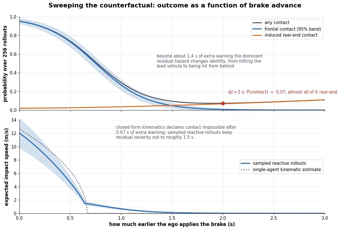
Two stacked charts against how much earlier the brake is applied. The upper chart plots probability of any contact, frontal contact with a confidence band, and rear-end contact over 256 rollouts, with frontal risk falling from near one to near zero and rear-end risk rising slowly. The lower chart plots expected impact speed from sampled reactive rollouts against a dotted single-agent kinematic estimate that reaches zero at 0.67 seconds

Figure 3: Sweeping the intervention turns one question into a curve. Frontal risk collapses within about one second of extra warning while rear-end exposure grows, so past roughly 1.4 s the dominant residual hazard has changed identity. The dotted line shows why sampling matters: the single-agent kinematic estimate declares the crash impossible after 0.67 s, whereas reactive rollouts still assign residual severity out to about 1.5 s.

Property	Log replay (non-reactive)	Rule-based reactive agents	Learned world model
Neighbour behaviour	Frozen to the recorded trajectory, blind to the new ego action	Car-following and lane-change heuristics with hand-set reaction times	Sampled from a learned conditional distribution over joint futures
Valid horizon	Only until the ego state diverges, often under 0.5 s	Seconds, as long as the manoeuvre stays inside the rule set	Seconds to tens of seconds, limited by compounding rollout error
What is simulated	Ego dynamics only, on ground-truth perception	Ego plus abstract agent boxes, still on ground-truth perception	Trajectories, occupancy, LiDAR, or camera frames, so perception can be tested in the loop
Cost per rollout	Negligible, millions of segments per night	Milliseconds, fully parallel across scenarios	Accelerator seconds per simulated second for generative sensor rollouts
Dominant failure mode	Fabricated collisions and hidden near misses	Over-polite traffic that inflates avoidance rates	Hallucinated agents, causal confusion, and quiet drift out of distribution
Best used for	Regression checks on planner outputs in unchanged scenes	Large-scale sweeps and worst-case bounds with auditable assumptions	High-stakes crash reconstruction and long-tail scenario editing

August 19, 2026

DL0158 3D-Aware World Model Geometry

How do 3D-aware latent world models use geometric inductive biases such as 3D Gaussian Splatting and NeRFs to ensure view-consistent camera rollouts?

Answer

A 3D-aware world model never lets a decoder invent pixels directly. Its latent transition predicts a scene state (a set of anisotropic 3D Gaussians, or the weights and features of a radiance field), and the only path from that state to an image is a differentiable renderer that takes the camera extrinsics and intrinsics as explicit arguments. Because every frame of a rollout is a deterministic function of one shared geometry, parallax, occlusion ordering, and disparity are produced by projection math rather than learned from data, so a camera can orbit for hundreds of steps without the scene mutating underneath it. NeRF contributed the volumetric rendering equation that made this pipeline differentiable end to end. 3D Gaussian Splatting keeps exactly the same alpha-compositing math but replaces per-ray marching with tile-based rasterization, which cuts per-frame cost by two to three orders of magnitude and is what makes closed-loop, interactive camera rollouts possible at all. The bias is not free: it guarantees consistency only where geometry is supported, so unobserved regions, topology changes, and strong view-dependent effects still require a generative prior layered on top.

(1) Render, Do Not Predict: the decoder is replaced by $\mathcal{R}(\mathcal{S}_t, \pi_t)$ , so the camera pose enters as a projection matrix instead of a conditioning token the network may ignore.
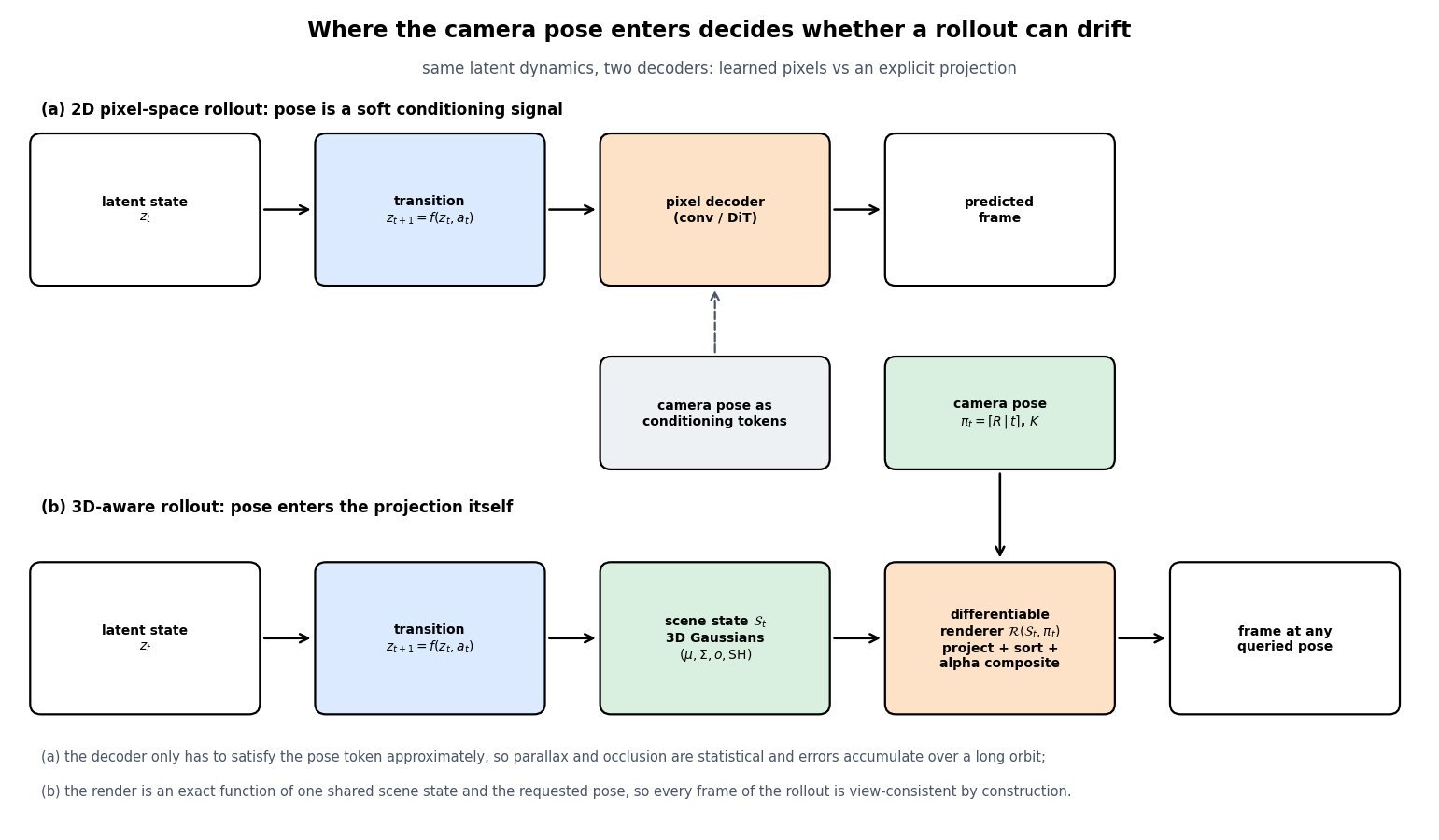
(2) One State, Many Views: all views share a single geometry, which turns multi-view consistency from a learned behaviour into an architectural invariant up to the representation’s capacity.
(3) Two Renderers, One Equation: NeRF integrates density along rays while 3DGS rasterizes projected Gaussians, but both use the same front-to-back alpha compositing, so the geometric bias is identical and only the cost model differs.
(4) Dynamics Live In Scene Space: time is handled by a deformation field or 4D Gaussians that move primitives, so motion cannot silently destroy the identity of an object the way pixel-space prediction can.
(5) Latency Decides Feasibility: a world model must render inside the control loop, and rasterization at roughly 5-10 ms per 1080p frame versus seconds for vanilla volumetric marching is the difference between a usable simulator and an offline reconstruction.
(6) Where The Bias Stops Helping: unobserved regions, non-rigid topology change, transparency, and monocular scale ambiguity are outside the guarantee and are exactly where a generative prior must take over.

Two-row architecture comparison. The top row shows a latent state feeding a transition function then a 2D pixel decoder that emits a predicted frame, with camera pose supplied only as conditioning tokens through a dashed arrow. The bottom row shows the same latent state and transition producing an explicit scene state of 3D Gaussians with position, covariance, opacity and spherical harmonics, which passes through a differentiable renderer that projects, sorts and alpha-composites, with the camera pose entering as extrinsics and intrinsics, emitting a frame at any queried pose.

Figure 1: The same latent dynamics, two decoders. In the pixel-space path the pose is a soft conditioning signal the decoder may only approximately honour, so geometric errors compound across a long orbit. In the 3D-aware path the pose is an argument of an exact projection, so consistency holds by construction and the model’s remaining job is predicting geometry rather than predicting appearance.

The mechanism that actually enforces consistency is worth stating precisely. A pixel is a function of the primitives that project onto it, sorted by depth, so moving the camera changes the projected position of a primitive by an amount inversely proportional to its depth. That single fact gives the renderer correct parallax, correct occlusion ordering when a near primitive covers a far one, and correct disocclusion when the camera slides sideways, all without any of it appearing in the loss as a special term. Training only needs a photometric loss on the observed views; the geometry that explains several views simultaneously is the only geometry that can drive that loss to zero, which is why a well-fit scene state extrapolates to nearby unseen poses. A 2D video model has to learn the same relationships as correlations over pixels, and it has no mechanism preventing a later frame from contradicting an earlier one.

Left panel is a top-down view of a scene with two camera poses at the bottom, dotted view frustums, a near orange elliptical splat at depth 2.8 and a far blue elliptical splat at depth 5.6, with solid rays drawn from each camera to each splat centre. Right panel shows the two resulting image strips stacked vertically, with orange and blue markers at the projected horizontal positions, and two double-headed arrows measuring that the near splat shifts 0.73 of the frame width between the views while the far splat shifts only 0.37, a ratio of exactly two matching the depth ratio.

Figure 2: Why a shared 3D state is a hard constraint. Both renders come from one set of primitives, so the horizontal shift of each splat is fixed by its depth: the near splat moves exactly twice as far as the splat at twice the distance. A pixel-space decoder must reproduce this ratio from statistics, whereas the renderer cannot violate it, which is the entire content of the phrase geometric inductive bias.

Mathematical Formulation:
$z_{t+1} = f(z_t, a_t)$
$\mathcal{S}_t = g(z_t)$
$I_t = \mathcal{R}(\mathcal{S}_t, \pi_t)$

Shared Rendering Equation:
$C(p) = \sum_{i=1}^{N} T_i \alpha_i c_i$
$T_i = \prod_{j=1}^{i-1} (1 - \alpha_j)$
$\alpha_i^{\mathrm{nerf}} = 1 - \exp(-\sigma_i \delta_i)$
$\alpha_i^{\mathrm{gs}} = o_i \, G_i(p)$
$\Sigma = R S S^{\top} R^{\top}$
$\Sigma' = J W \Sigma W^{\top} J^{\top}$
$\mu_i(t) = \mu_i + \Delta\mu_i(z_t)$

Where:

$z_t$ is the compact latent state, $a_t$ the action, and $f$ the learned transition model; $g$ decodes the latent into a scene state rather than into pixels.
$\mathcal{S}_t$ is the geometric state: for 3DGS a set of primitives $\{\mu_i, \Sigma_i, o_i, \mathrm{SH}_i\}$ , for a NeRF a field returning density and colour at a queried point and direction.
$\pi_t = (R \mid t, K)$ is the camera pose and intrinsics, and $\mathcal{R}$ the differentiable renderer; $I_t$ is the frame, so any pose can be queried at any rollout step.
$C(p)$ is the colour of pixel $p$ , $i$ indexes the $N$ contributions sorted front to back, $c_i$ is the view-dependent colour, and $T_i$ is the accumulated transmittance that produces occlusion for free.
$\sigma_i$ is the volume density at sample $i$ and $\delta_i$ the spacing between adjacent samples along the ray; $o_i$ is a Gaussian’s opacity and $G_i(p)$ its projected 2D density evaluated at the pixel.
$\Sigma$ is the world-space covariance factored into rotation $R$ and scale $S$ so it stays positive semi-definite under gradient descent, and $\Sigma'$ is its screen-space projection through the viewing transform $W$ and the affine Jacobian $J$ .
$\Delta\mu_i(z_t)$ is the predicted per-primitive displacement from a canonical configuration, which is how dynamics enter without breaking the static consistency guarantee at each instant.

The cost model is what selects the representation in practice. Volumetric marching evaluates a network at every sample on every ray, so a vanilla NeRF pays roughly $2 \times 10^{6}$ rays times 192 samples for one 1080p frame, which is hundreds of millions of queries. Hash-grid encodings shrink the per-query cost by orders of magnitude but keep the same per-ray structure. Rasterization instead touches each Gaussian once, splats it into the tiles it covers, and blends sorted contributions, which turns rendering into a bandwidth-bound pass rather than a compute-bound integral. That is the reason 3D-aware world models became practical after 2023 rather than after 2020.

Log-log line chart of milliseconds per frame versus output resolution in megapixels for three renderers: vanilla NeRF with 192 samples per ray at about 47000 milliseconds per megapixel, a hash-grid accelerated field at about 15 milliseconds per megapixel, and 3D Gaussian rasterization at about 3.7 milliseconds per megapixel, with horizontal reference lines at the 33 millisecond thirty frames per second budget and the 11 millisecond ninety frames per second budget, and an annotation marking that rasterization renders 1080p in roughly 8 milliseconds.

Figure 3: The geometric bias is only usable if you can afford to render. All three curves are linear in pixel count, so the gaps are constant multipliers: rasterization clears the 33 ms interactive budget at 1080p with room to spare, a hash-grid field sits near the edge, and vanilla volumetric marching is four orders of magnitude away, which restricts it to offline reconstruction rather than in-the-loop camera rollouts.

Property	2D latent video world model	NeRF-style radiance field	3D Gaussian splats
Scene representation	Latent tokens or 2D feature maps, no explicit geometry	Implicit continuous field returning density and colour	Explicit primitives with position, covariance, opacity, spherical harmonics
How the camera enters	Conditioning embedding, a soft constraint the decoder can bend	Defines ray origins and directions used for sampling	Enters the viewing transform and the projection Jacobian
Cost per 1080p frame	One pass of a large decoder, tens to hundreds of ms	Seconds for a vanilla MLP field, tens of ms with hash grids	Single rasterization pass, roughly 5-10 ms
View consistency	Statistical, drifts as the orbit lengthens	Exact for supported geometry	Exact for supported geometry, same compositing math
Dynamics	Native, learned directly in latent or pixel space	Time-conditioned field or canonical space plus deformation	Per-primitive deformation or 4D Gaussians
Dominant failure mode	Hallucinated geometry and object identity flicker on return views	Slow to fit and render, blurry thin structures, hard to edit	Floaters and popping in unobserved regions, memory grows with primitive count

August 19, 2026