Tag: WorldModel

Action-conditioned and generative world models

DL0150 Generative Multi-View World Model

How do generative world models generate realistic, high-resolution multi-view camera outputs (e.g., 8 ring cameras on a vehicle) with spatial and temporal coherence?

Answer

Modern driving world models are latent video diffusion models rather than per-camera image generators. A causal video tokenizer compresses every camera stream (roughly 16x spatially and 4x temporally), and one diffusion transformer denoises a single latent tensor that holds all 8 views and all frames of the clip simultaneously, so coherence is a property of the sampling process instead of a post-hoc fix. Spatial agreement between neighbouring cameras comes from two ingredients: cross-view attention inside every block, and camera-geometry conditioning that tells each token where its camera points, usually as per-pixel Plücker ray embeddings built from the intrinsics and extrinsics of that rig. Temporal agreement comes from a temporal attention axis plus a shared ego-action and agent-layout condition that all 8 views must obey, so a braking maneuver or a crossing pedestrian appears in every camera at the same instant. High resolution is bought with a cascade instead of brute force: the transformer works in a small latent grid, and a separate diffusion upsampler restores full per-view pixels, while long horizons come from autoregressive rollout over overlapping context frames.

(1) Latent, Not Pixel, Diffusion: a learned video tokenizer removes most spatial and temporal redundancy first, so the generator never denoises 8 megapixel-scale streams directly.
(2) One Joint Tensor Over Views And Time: the state being denoised is $z \in \mathbb{R}^{V \times T \times N \times c}$ , which is why views cannot drift into independent hallucinations.
(3) Factorized 4D Attention: spatial attention within a view-frame, cross-view attention across the ring at a fixed time, and temporal attention across time within a view, roughly 126x cheaper than full joint attention at 8 views and 16 frames.
(4) Geometry As A First-Class Condition: Plücker rays per pixel (plus optional epipolar-constrained attention) let one model serve rigs with different camera counts, mounting positions, and fields of view.
(5) Shared Layout And Action Control: 3D agent boxes, an HD map or BEV raster, and the ego trajectory are broadcast to every view, so all cameras render the same world state rather than eight plausible worlds.
(6) Cascade And Rollout: a super-resolution diffusion stage supplies pixels and an overlapped sliding window supplies duration, at the cost of error accumulation over long horizons.

Pipeline diagram: eight-view video enters a causal video tokenizer with 16x spatial and 4x temporal compression, producing a latent grid of V by T by N tokens that feeds a diffusion transformer of L blocks, then a latent decoder and a diffusion upsampler back to 448 by 960 per view; an expanded panel shows one block containing spatial self-attention within a view-frame, cross-view attention across the eight views at one time step, and temporal attention across frames of one view, with camera Plucker rays, ego action, agent layout, and noise level injected on the right

Figure 1: One tokenizer, one transformer, one upsampler. The only thing that makes this a multi-view model rather than eight video models is the cross-view attention axis and the shared conditioning bundle; the token budget of 215,040 latents per clip is what forces the attention to be factorized.

The cross-view axis is where naive designs fail, and geometry explains why. Ring cameras overlap only with their immediate neighbours, so attending from the rear camera to the front camera buys almost nothing while costing the same as a useful pair; restricting cross-view attention to ring-adjacent views keeps essentially all of the benefit. Inside an adjacent pair, a point visible in view $i$ cannot be anywhere in view $j$ : the fundamental matrix of the calibrated rig confines it to a single epipolar line, which is why epipolar-band attention is a legitimate sparsification rather than a heuristic. Conditioning carries the rest of the load. Because the ego action and the 3D agent boxes are shared, the front-left and front cameras are both being asked to render the same car at the same metric position, and the overlap region then agrees on colour, exposure, geometry, and occlusion because both views were denoised from the same layout under attention that could compare them at every layer.

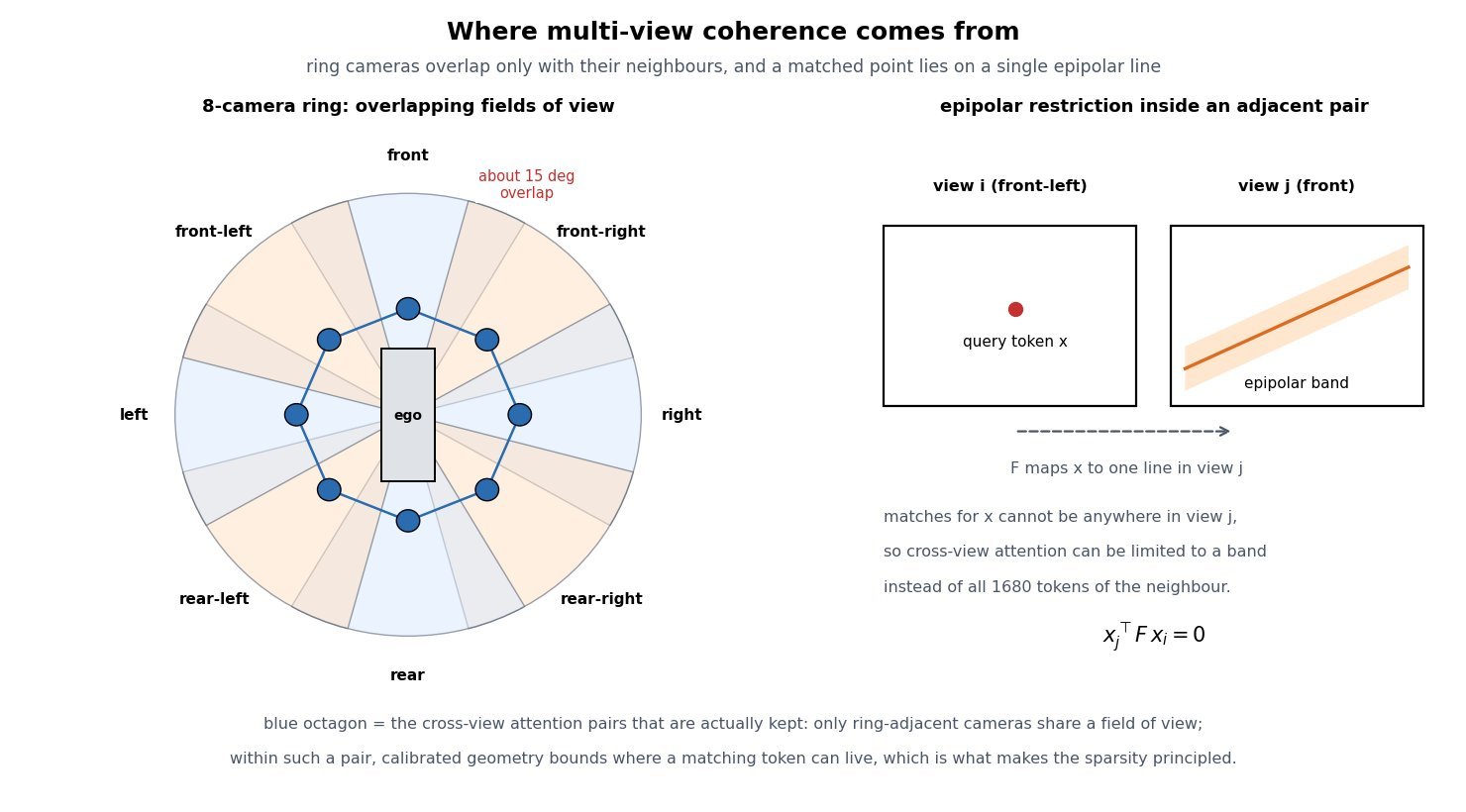
Left panel: top-down view of a vehicle with eight camera field-of-view wedges arranged in a ring, labelled front, front-right, right, rear-right, rear, rear-left, left, and front-left, with a 15 degree overlap marked between neighbours and an octagon of lines connecting adjacent camera nodes to show which pairs exchange cross-view attention. Right panel: two image-plane rectangles for view i and view j, a marked point x in view i and the corresponding epipolar band drawn as a shaded stripe in view j, with the constraint that a matching token lies on that single line.

Figure 2: Coherence is a geometry problem before it is a modelling problem. Only ring-adjacent pairs share a field of view, and within a pair the epipolar constraint bounds where a matching token can live, so both the sparsity pattern and the conditioning signal are dictated by the calibrated rig.

Mathematical Formulation:
$z \in \mathbb{R}^{V \times T \times N \times c}$
$N = (H/p)(W/p) = 28 \times 60 = 1680$
$L = V T N = 8 \times 16 \times 1680 = 215040$
$\mathcal{L}(\theta) = \mathbb{E}\left[\lVert \epsilon - \epsilon_{\theta}(z_t, t, c) \rVert^2\right]$
$c = (r, a, b, z_{\mathrm{ctx}})$
$r_{uv} = (d_{uv},\ o \times d_{uv}) \in \mathbb{R}^{6}$

Where:

$z$ is the joint latent tensor being denoised, with $V=8$ views, $T$ latent frames, $N$ tokens per view-frame, and $c$ latent channels.
$H \times W = 448 \times 960$ is the per-view pixel resolution and $p = 16$ the combined tokenizer and patch downsampling factor, giving a $28 \times 60$ latent map.
$L$ is the total sequence length if the clip were flattened, the number that decides whether full attention is affordable.
$\epsilon$ is the sampled noise, $z_t$ the noised latent at level $t$ , and $\epsilon_{\theta}$ the diffusion transformer.
$c$ bundles the conditioning: per-view rays $r$ , ego action $a$ (speed and curvature), agent and map layout $b$ , and the overlapping context latents $z_{\mathrm{ctx}}$ from the previous window.
$r_{uv}$ is the Plücker embedding of the ray through pixel $(u,v)$ , with unit direction $d_{uv}$ and camera origin $o$ , so extrinsics and intrinsics enter as a 6-channel image instead of a flat vector.

Attention Cost Per Block:
$C_{\mathrm{full}} = L^2 = 4.62 \times 10^{10}$
$C_{\mathrm{spa}} = V T N^2 = 3.61 \times 10^{8}$
$C_{\mathrm{view}} = T N V^2 = 1.72 \times 10^{6}$
$C_{\mathrm{tmp}} = V N T^2 = 3.44 \times 10^{6}$
$C_{\mathrm{spa}} + C_{\mathrm{view}} + C_{\mathrm{tmp}} = 3.66 \times 10^{8}$

Factorization therefore costs about 0.8% of full joint attention at this shape, and almost all of the remaining cost is ordinary within-frame spatial attention. The cross-view and temporal axes together add under 1.5% on top of the spatial term, which is the practical reason multi-view coherence is affordable at all: the expensive part of the model is generating each image, not keeping the images consistent.

Log-scale line chart of attention pairs per transformer block against the number of camera views from 1 to 8, with 16 latent frames and 1680 tokens per view-frame. The full joint 4D attention curve rises quadratically from about 7.2e8 to 4.62e10 pairs, while the factorized spatial plus cross-view plus temporal curve rises nearly linearly from about 2.9e7 to 3.66e8 pairs, an annotation noting the roughly 126x gap at eight views.

Figure 3: Full joint attention over the flattened clip grows as $V^2$ while the factorized form grows close to linearly in $V$ , so the gap widens with every camera added to the rig. Adding a ninth or tenth view is a routine cost in the factorized design and prohibitive in the joint one.

Property	Independent per-view generation	Factorized view + time attention	Full joint 4D attention
Attention pairs per block	3.61e8 (spatial only)	3.66e8, about 1.4% overhead	4.62e10, roughly 126x more
Overlap agreement	None; only the shared layout condition, so seams disagree	Enforced on ring-adjacent pairs, optionally epipolar-banded	Enforced globally, mostly on pairs that never overlap
Temporal behaviour	Per-view only; the eight views desynchronize over rollout	Temporal axis plus one shared action keeps views in lockstep	Strongest in principle, but memory caps the clip length
Failure signature	Objects appear in one camera and vanish in its neighbour	Slow drift of far-field content and appearance across rollout	Out-of-memory or a clip too short to be useful for simulation
Practical verdict	Useless for BEV or occupancy training data	The production choice for ring-camera world models	Research ablation at small resolution or few frames

August 18, 2026

DL0149 World Models from Unlabeled Video

How do world models learn interactive, action-controllable environment rollouts from unlabeled video datasets without ground-truth action labels?

Answer

The missing action labels are invented by the model itself. A latent action model (LAM) is an inverse-dynamics encoder that looks at the past frames and the next frame together and emits a single discrete code $z_t$ through a vector-quantized bottleneck; a forward dynamics model is then required to predict that next frame from the past frames plus $z_t$ alone. Both halves are trained jointly with next-frame reconstruction as the only supervision, so the code is pushed to carry exactly the part of the transition that the past cannot explain, which for gameplay and egocentric video is precisely the agent’s action. Genie made this concrete at scale, training an 11B-parameter model on roughly 30,000 hours of filtered 2D platformer video with a codebook of only $K = 8$ latent actions, and the tiny codebook is not a detail but the mechanism: at 3 bits per step the code physically cannot smuggle the next frame through it. At inference the LAM encoder is thrown away, a key press is mapped onto one of the $K$ learned codes, and the dynamics model rolls the world forward autoregressively, which turns passive video into a playable environment.

(1) Latent Action Model: an inverse-dynamics encoder over $(x_{1:t}, x_{t+1})$ produces one discrete code per transition, standing in for the action label that the dataset never had.
(2) The Bottleneck Is The Whole Trick: a codebook of size $K = 8$ caps the code at $\log_2 8 = 3$ bits, forcing it to describe a control decision rather than pixels.
(3) Reconstruction Is The Only Loss: the forward model’s next-frame error trains the encoder through the quantizer, so no human ever annotates a button.
(4) Tokenize, Then Roll Out: a spatiotemporal VQ-VAE turns frames into tokens and a masked-token or diffusion dynamics model generates the next frame conditioned on the past tokens and $z_t$ .
(5) Codes Are Shared Across Videos: because one codebook serves the whole corpus, the same index means the same intent in unseen scenes, which is what makes the latent space a controller instead of a per-clip artifact.
(6) Grounding To Real Controls Is Cheap: a handful of labeled clips, or human probing of each code, suffices to attach semantics; VPT instead spent 2,000 labeled hours to train an inverse-dynamics model and pseudo-labeled 70,000 web hours with it.
(7) Rollouts Drift: generation is autoregressive on its own output, so compounding error, memory loss, and entangled camera-versus-agent motion dominate the failure list.

Two-panel diagram. The training panel shows past frames and the next frame both entering a latent action model with a VQ bottleneck of eight codes, producing a 3-bit code, while the past frames are separately tokenized by a spatiotemporal VQ-VAE; both streams enter a masked video-token dynamics model whose only loss is reconstruction of the next frame. The inference panel shows a key press selecting one of the eight codes without the latent action model, feeding the same dynamics weights, decoding and rendering a frame that loops back as the next context.

Figure 1: The asymmetry between the two panels is the point. During training the next frame is visible to the latent action model, which is why an unlabeled corpus can supervise a controller; at inference that encoder is discarded and the codebook itself becomes the input device, with the rendered frame fed back as context for the next step.

Everything hinges on how much information the quantizer lets through. If the latent is generous (a wide continuous vector, or a codebook of thousands of entries), the encoder discovers the shortcut of encoding the next frame directly, the dynamics model degenerates into a decoder of the latent, reconstruction looks excellent, and controllability collapses because a user-chosen code no longer corresponds to anything an agent could do. If the latent is too narrow, distinct moves collapse into one code and the environment responds to only a couple of coarse commands. The standard diagnostic is a controllability delta: roll the model forward with the inferred code, then with a random code, and measure the gap in frame quality. A large gap means the code is doing real work; a gap near zero means either leakage or a code the model ignores.

Mathematical Formulation:
$z_t = q(f_{\phi}(x_{1:t+1}))$
$\hat{x}_{t+1} = g_{\theta}(x_{1:t}, z_t)$
$\mathcal{L}(\phi,\theta) = \| x_{t+1} - \hat{x}_{t+1} \|_2^2$
$H(z_t) \leq \log_2 K$
$\Delta = \mathrm{PSNR}(z_t) - \mathrm{PSNR}(\tilde{z})$

Where:

$z_t$ is the latent action for the transition at step $t$ , and $q$ is vector quantization onto a codebook of $K$ entries.
$f_{\phi}$ is the inverse-dynamics encoder, which is the only component allowed to see the future frame, and $\phi$ are its parameters.
$x_{1:t}$ are the observed past frames (in practice their VQ tokens), $x_{t+1}$ is the true next frame, and $\hat{x}_{t+1}$ is the prediction.
$g_{\theta}$ is the forward dynamics model, a masked video-token transformer or a diffusion decoder, conditioned on the past plus $z_t$ and nothing else.
$\mathcal{L}$ is the reconstruction objective, extended in practice by the usual commitment and codebook terms; no action label appears in it, which is why unlabeled video is sufficient.
$H(z_t) \leq \log_2 K$ is the capacity bound that prevents frame leakage, giving 3 bits per step when $K = 8$ .
$\Delta$ is the controllability metric, comparing a rollout driven by the inferred code against one driven by a random code $\tilde{z}$ drawn from the same codebook.

Why 3 Bits Cannot Encode A Frame:
$\log_2 K = \log_2 8 = 3 \ \text{bits}$
$256 \times 10 = 2560 \ \text{bits per frame}$

A $16 \times 16$ token grid over a 1024-entry visual codebook already carries about 2,560 bits, roughly three orders of magnitude more than the action code, so the encoder has no route to cheat and the dynamics model must genuinely keep a model of the scene in its context. That ratio is the design knob you actually tune: too small and the environment is unresponsive, too large and it stops being an environment at all.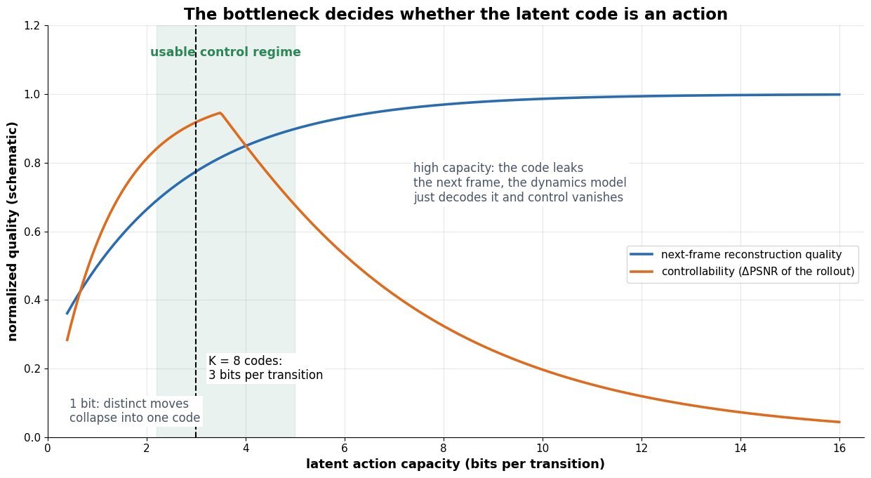

Schematic line chart with latent action capacity in bits per transition on the x-axis and normalized quality on the y-axis. Next-frame reconstruction quality rises monotonically and saturates, while controllability rises to a peak near three bits and then decays toward zero as capacity grows, with a shaded band marking the usable control regime between about two and five bits and a dashed vertical line at three bits labeled as an eight-entry codebook.

Figure 2: Schematic view of the tension that a single reconstruction loss hides. Reconstruction quality never warns you about failure because it keeps improving as the latent widens, whereas controllability peaks and then collapses once the code can carry the frame; only the two curves together tell you the bottleneck is set correctly.

Property	Latent action model (no labels)	Inverse-dynamics pseudo-labeling	Logged true actions
Label requirement	None during training; a few clips only to name the codes	A labeled seed set, such as VPT’s 2,000 contractor hours	Every frame paired with the true control input
Action space	Discovered discrete codes, semantics unknown a priori	The real action API, recovered by a trained predictor	The real action API, exactly
Data ceiling	Any internet video of the domain	Any video, but the seed set must match the domain	Only instrumented environments and agents
Dominant failure mode	Frame leakage through a wide latent, or codes entangling camera and agent motion	Pseudo-label noise on rare actions propagates into the dynamics	Coverage limited to the logging policy’s behaviour
Representative system	Genie, LAPO	VPT	GameNGen, Dreamer-style agents

August 18, 2026

DL0125 Action-Conditioned World Model

Explain the architecture of an Action-Conditioned World Model for autonomous driving, of the kind Wayve describes for its GAIA models.

Answer

An action-conditioned world model is a generative model of future sensor data whose predictions are explicitly steered by the ego vehicle’s own control commands, so it can answer “what would the road look like in three seconds if I brake at 5 m/s² instead of holding speed?”. Architecturally it factors into four blocks that are trained in two stages: a video encoder that compresses multi-camera frames into a small latent grid, an action and context encoder that embeds the low-dimensional control signal, a latent dynamics model that rolls the compressed state forward in time, and a decoder plus auxiliary heads that render latents back to pixels or BEV occupancy. Almost every production-scale system follows this shape and differs only in the dynamics block: GAIA-1 uses a 6.5B-parameter causal transformer over discrete video tokens with a separate diffusion video decoder, GAIA-2 replaces it with a flow-matching diffusion transformer over continuous latents so five surround views stay geometrically consistent, and Dreamer-style recurrent state-space models keep a compact deterministic-plus-stochastic state for reinforcement learning in imagination. The reason compression comes first is the same as in latent diffusion: at 6.25 Hz a 26-frame context of $288 \times 512$ frames is 3.8M pixels per frame-stack but only 14,976 latent tokens, and the dynamics model’s cost is quadratic in that number. What makes the model a simulator rather than a video generator is the rollout loop plus faithful action adherence, which is precisely where these models are weakest and where interviewers push.

(1) Observation Encoder: a VQ or KL-regularized video autoencoder with spatial factor $f = 16$ to $32$ maps each frame to an $18 \times 32$ grid; it is trained first with perceptual and adversarial losses, then frozen.
(2) Action And Context Conditioning: a 2-D action (curvature and acceleration) is embedded by a small MLP and injected per frame at every block, as prefix tokens or through AdaLN modulation, alongside text prompts, agent bounding boxes, and camera calibration.
(3) Latent Dynamics Backbone: a causal spacetime transformer predicting the next token, or a diffusion/flow-matching transformer denoising a whole latent chunk conditioned on the past; this is where nearly all parameters live.
(4) Decoder And Auxiliary Heads: a diffusion or convolutional decoder for video, plus cheap heads for BEV occupancy, collision cost, and value that planning actually consumes.
(5) Two-Stage Training With Teacher Forcing: the dynamics model always sees ground-truth latents during training, which creates the exposure-bias gap that dominates long-horizon rollouts.
(6) Three Consumers: closed-loop policy evaluation against counterfactual actions, planning or RL in imagination, and generation of rare corner-case scenarios that fleets rarely log.

Left to right pipeline: five surround cameras feed a video tokenizer producing an 18 by 32 latent per frame, a dynamics transformer conditioned on action, text, agent boxes and camera pose predicts future latents with an autoregressive rollout loop, and a decoder renders predicted video and BEV occupancy

Figure 1: The four blocks of an action-conditioned world model. Only the frozen codec ever touches pixels, the action modulates every block of the dynamics model, and the rollout loop is what turns a video generator into a driving simulator.

How the action enters is the part worth rehearsing. A two-number control signal has to influence a token stream dominated by appearance, so injecting it once at the input is not enough: it is embedded per frame and re-applied at every layer, and it must be time-aligned to the interval it causes rather than the frame it was logged with. Two failure modes follow directly. First, shortcut learning: logged actions are almost perfectly predictable from the visible road geometry, so a model can minimize training loss while ignoring $a_t$ entirely, and you only detect this by rolling out counterfactual actions that contradict the scene. Second, weak controllability at sampling time, which is why conditioning is dropped for 10-20% of training samples so that classifier-free guidance can later amplify action adherence. Evaluation therefore needs an action-following metric (does the rendered ego trajectory match the commanded one?) next to FID or FVD, because generative realism and control fidelity move independently.

Mathematical Formulation:
$z_t = \mathcal{E}(o_t)$
$h_t = f_\theta(h_{t-1}, z_{t-1}, a_{t-1})$
$\hat{z}_t \sim p_\theta(z_t \mid h_t, a_{t-1})$
$\hat{o}_t = \mathcal{D}(h_t, \hat{z}_t)$
$\mathcal{L} = \mathcal{L}_{\text{obs}} + \beta \, \mathcal{L}_{\text{dyn}}$
$\mathcal{L}_{\text{obs}} = -\log p_\theta(o_t \mid h_t, z_t)$
$\mathcal{L}_{\text{dyn}} = D_{KL}\!\left(q_\phi(z_t \mid h_t, o_t) \,\|\, p_\theta(z_t \mid h_t)\right)$
$p(z_{1:T} \mid a_{1:T}) = \prod_{t=1}^{T} p(z_t \mid z_{1:t-1}, a_{1:t-1})$
$N = T \cdot (H/f) \cdot (W/f)$
$N = 26 \cdot 18 \cdot 32 = 14{,}976$

Where:

$o_t$ is the multi-camera observation at step $t$ and $\hat{o}_t$ its prediction; $a_t$ is the ego action (curvature and acceleration, or steering and pedal).
$z_t$ is the compressed observation latent and $h_t$ the deterministic recurrent or attention-carried state that summarizes the past.
$\mathcal{E}$ and $\mathcal{D}$ are the frozen encoder and decoder, $f_\theta$ the dynamics backbone, $p_\theta$ the action-conditioned prior, and $q_\phi$ the posterior that also sees the true observation.
$\beta$ balances reconstruction against the dynamics (KL) term; in practice it is annealed and often free-bits clipped so the prior does not collapse onto the posterior.
$T$ is the context length in frames, $H \times W$ the frame resolution, $f$ the spatial compression factor, and $N$ the token count whose square drives attention cost.
Required initial conditions for a rollout: $h_0 = 0$ and a real context $z_{1:k}$ encoded from logged frames, after which only actions are supplied and $j > k$ steps are pure imagination.

Left panel: bird's-eye view of three ego trajectories branching from the same start under hold-speed, brake and lane-change action sequences, with a braking lead vehicle and a predicted collision marker. Right panel: prediction error versus rollout horizon for one-step re-encoding, free-running rollout, and a variant with action tokens ablated

Figure 2: Left: fixing the initial latent and varying only the action sequence produces counterfactual rollouts, the property that makes the model usable for closed-loop evaluation. Right: because training is teacher-forced, free-running error compounds superlinearly, and ablating the action tokens makes it worse still.

Dynamics block	Discrete-token autoregressive	Latent diffusion / flow matching	Recurrent state-space (RSSM)
Latent representation	VQ codebook indices, 576 tokens per frame	Continuous latent grid, tens of channels, temporally compressed	Small vector state: deterministic GRU plus categorical stochastic units
How the action enters	Per-frame prefix tokens in the causal sequence	AdaLN modulation or cross-attention at every block, with conditioning dropout	Concatenated into the recurrent transition at each step
Rollout cost	Hundreds of sequential token decodes per frame; slowest	Tens of denoising steps per chunk, parallel across positions	One cheap matrix step per frame; fast enough for RL in imagination
Strength	Exact likelihoods, easy long-context scaling, LLM tooling reuse	Best photorealism and multi-view consistency; controllable via guidance	Compact enough to train a policy on millions of imagined steps
Typical failure mode	Quantization artifacts and drift after a few seconds of rollout	Plausible but unfaithful scenes; ignores the action unless guided	Blurry reconstructions; posterior collapse hides rare agents
Representative system	GAIA-1	GAIA-2, Vista, NVIDIA Cosmos	DreamerV3, MILE

August 17, 2026

DL0124 3D Occupancy Flow

What is 3D Occupancy Flow? What is the tradeoff for predicting dense spatiotemporal occupancy grids instead of discrete 3D bounding-box trajectories?

Answer

3D Occupancy Flow is a joint perception-and-forecasting output format that replaces the list of tracked objects with a dense grid: for every voxel (or BEV cell) and every future waypoint the network predicts an occupancy probability plus a flow vector describing how the mass in that cell moves. Waymo’s Occupancy Flow Fields formulation predicts three quantities per waypoint on a $256 \times 256$ BEV grid covering roughly $80\ \text{m} \times 80\ \text{m}$ : observed occupancy, occluded occupancy, and backward flow. Camera-only 3D variants such as Occ3D on nuScenes predict a $200 \times 200 \times 16$ voxel grid at $0.4\ \text{m}$ resolution, and Tesla presented an occupancy network with an occupancy-flow head at its 2022 AI Day. The appeal is that free space and obstacle geometry become class-agnostic and non-parametric: a tipped-over mattress, an articulated trailer, a swinging crane boom, and an overhanging branch all get represented without appearing in a detector taxonomy, and probability mass can sit on both branches of a fork at once without a mode head or non-maximum suppression. The cost is that a grid has no notion of an object, so instance identity, track continuity, and per-agent attributes disappear, and the output tensor grows by roughly two orders of magnitude, which pushes cost onto compute, memory, label pipelines, and the loss function’s handling of a grid where the overwhelming majority of voxels are empty. In practice this is why most production stacks run occupancy flow alongside a box pipeline rather than as a drop-in replacement.

(1) Dense Spatiotemporal Output: the head emits $o_t(v)$ and $f_t(v)$ for every cell and every future timestep, not a parametric box with a heading and a velocity per agent.
(2) Class-Agnostic Geometry: anything that occupies space is representable, which removes the long-tail detection failure where an unlisted object class becomes invisible to the planner.
(3) Backward Flow, Not Forward: predicting motion from $t$ back to $t-1$ makes warping a gather with one source per cell, so mass never collides during the warp and a flow-grounded occupancy consistency check becomes well defined.
(4) Non-Parametric Multimodality: a grid holds several futures simultaneously as spread probability mass, but that same property makes averaged modes look like blur or ghost occupancy rather than a ranked set of hypotheses.
(5) Identity Is What You Give Up: without instance IDs, right-of-way logic, interaction-aware conditioning, and per-object intent signals such as turn indicators lose their handle on the scene.
(6) Cost Scales With The Grid: output size grows as $H W D T$ , dense labels require multi-sweep LiDAR accumulation and voxelization, and roughly 95% or more of voxels are empty, so class imbalance dominates the occupancy loss.

Diagram contrasting two forecasting pipelines from the same sensor input: an object-centric branch running detector, tracker, and trajectory predictor to emit sparse box waypoints, and an occupancy-centric branch running a BEV or voxel encoder with occupancy and backward-flow heads to emit a dense spatiotemporal grid

Figure 1: The object-centric branch (detect → track → forecast) produces a sparse, identity-carrying output limited by its taxonomy; the occupancy branch skips detection and data association entirely and produces a dense, class-agnostic grid with no instance IDs.

The deeper tradeoff is not really compute, it is what the downstream planner can express. A box trajectory is a commitment: this vehicle, with this ID, will be here in 3 seconds with this probability, which lets a planner reason about yielding to a specific agent, replay a scenario in simulation, and produce an auditable explanation for a maneuver. Occupancy flow is a statement about space, which is exactly what collision checking and drivable-free-space queries want, but a grid that hedges between “the cyclist goes straight” and “the cyclist turns” paints both corridors at moderate probability, and a naive cost function that treats any occupancy above a threshold as blocked yields the freezing-robot behavior. Occupancy flow partially recovers correspondence without identity: warping the previous occupancy along the predicted backward flow and multiplying it against the current occupancy gives a differentiable consistency term, so the model is penalized for teleporting mass even though it never names an object.

Mathematical Formulation:
$0 \leq o_t(v) \leq 1$
$\hat{o}_t = o_t \odot \mathcal{W}(o_{t-1}, f_t)$
$\mathcal{L} = \mathcal{L}_{occ} + \lambda \mathcal{L}_{flow}$
$\mathcal{L}_{occ} = \sum_{t=1}^{T} \sum_{v} \mathrm{BCE}(o_t(v), y_t(v))$
$\mathcal{L}_{flow} = \sum_{t=1}^{T} \sum_{v \in \Omega_t} \lVert f_t(v) - f_t^{*}(v) \rVert_1$
$N_{occ} = 200 \cdot 200 \cdot 16 \cdot 8 = 5.12 \times 10^{6}$
$N_{box} = 50 \cdot 6 \cdot 16 \cdot 5 = 2.40 \times 10^{4}$

Where:

$o_t(v)$ is the predicted occupancy probability of cell $v$ at future waypoint $t$ , and $f_t(v)$ is the backward flow vector pointing to where that mass sat at $t-1$ .
$\mathcal{W}$ is the warp operator that gathers $o_{t-1}$ along $f_t$ (bilinear or trilinear), and $\hat{o}_t$ is the flow-grounded occupancy used both as a loss term and as an evaluation metric.
$y_t(v)$ is the voxelized ground-truth occupancy label, $f_t^{*}$ the ground-truth flow, and $\Omega_t$ the set of genuinely occupied cells to which the flow loss is masked.
$t \in \{1, \ldots, T\}$ indexes waypoints and $v$ indexes the $H \times W \times D$ grid; $\lambda$ balances the two terms, and $\mathrm{BCE}$ is usually replaced by a focal or class-balanced variant because empty voxels dominate.
$N_{occ}$ counts predicted occupancy values for a $200 \times 200 \times 16$ grid over 8 waypoints, and $N_{box}$ counts a comparable box head with 50 agents, 6 modes, 16 waypoints, and 5 numbers per waypoint.
Required initial condition: $o_0$ and the whole grid must be expressed in the ego frame at $t = 0$ , so ego motion is compensated before flow is interpreted as agent motion.

Grid diagram showing occupancy at time t minus one in light dashed cells and predicted occupancy at time t in solid cells, with backward flow arrows drawn from each occupied cell at time t to the cell its mass came from, alongside the flow-grounded occupancy product equation

Figure 2: Backward flow assigns each occupied cell at time $t$ a single source cell at $t-1$ , so the warp is a gather rather than a scatter and the consistency product $o_t \odot \mathcal{W}(o_{t-1}, f_t)$ penalizes mass that appears without a plausible origin.

Resolution and horizon are the two knobs that make or break the design. Halving the voxel size multiplies the tensor by 8 in 3D, and every additional waypoint is another full grid, so a $0.2\ \text{m}$ grid over a 5-second horizon at $2\ \text{Hz}$ is far beyond a real vehicle compute budget once flow channels and semantics are added. Going the other way is not free either: at $0.4\ \text{m}$ voxels a pedestrian walking at $1.4\ \text{m/s}$ moves less than one voxel per $0.2\ \text{s}$ frame, so the flow target is sub-voxel and the occupancy channel alone cannot express the motion, which is precisely why the flow head is kept as a continuous regression rather than a discrete cell-to-cell assignment.

Log-scale bar chart of predicted output size per inference: 24000 numbers for multi-modal box trajectories, 524288 for a 256 by 256 BEV occupancy grid over 8 waypoints, 5.12 million for a 200 by 200 by 16 voxel grid over 8 waypoints, and 20.48 million once three flow channels are added

Figure 3: Output size is where the tradeoff becomes concrete: the 3D voxel grid predicts about 213x more numbers than a multi-modal box head, and adding a 3-channel flow field multiplies that by another 4 before any semantic classes are included.

Property	3D occupancy flow	Box trajectories	Hybrid stack
Output per inference	Millions of per-cell values, occupancy plus flow per waypoint	Tens of thousands of numbers, a few modes per tracked agent	Both, sharing one BEV or voxel backbone
Unlisted geometry	Represented, since occupancy is class-agnostic	Dropped if no detector class fits it	Covered by the occupancy branch
Instance identity	None; only flow-based correspondence	Explicit IDs, attributes, and track history	IDs from the box branch, geometry from the grid
Multimodality	Implicit in the probability field, no mode count to tune	Explicit ranked modes with confidences	Explicit modes for interaction, field for collision checks
Supervision	Accumulated multi-sweep LiDAR voxelized into dense labels	Human box and track annotations only	Both label pipelines must be maintained
Typical failure mode	Blurred or ghost occupancy that makes the planner over-conservative	Missed detection or ID switch removes an obstacle entirely	Disagreement between branches needs an arbitration policy

August 17, 2026

DL0122 V-JEPA vs Video World Models

Compare V-JEPA (Joint-Embedding Predictive Architecture) with video generation world models such as OpenAI’s Sora or NVIDIA Cosmos. What does each objective actually learn, and when would you deploy one over the other?

Answer

Both families are trained by predicting the unseen part of a video, and both are called world models, but they differ in where the prediction target lives. V-JEPA masks a large 3D region of a clip and trains a predictor to regress the embeddings of that region produced by an EMA target encoder, using an L1 loss in representation space; there is no decoder anywhere in the system, so the model is never asked to reproduce a pixel. Sora and Cosmos Predict instead train a generative model (a diffusion transformer over spacetime latent patches, or an autoregressive token model) to reconstruct the actual frames, which forces the network to spend capacity on every detail, including detail that is fundamentally unpredictable, such as the exact texture of foliage or the phase of a reflection. That single design choice cascades: V-JEPA gets a compact motion-aware representation and a rollout that costs one forward pass per step, which is what makes energy-based planning tractable, while generative world models get a renderable future that can serve as a simulator, a synthetic-data generator, or an input to an existing camera-based perception stack. Neither dominates; the question to ask in an interview is whether your downstream consumer is a policy or a pixel pipeline.

(1) Target Space: V-JEPA minimizes distance between predicted and EMA-encoded latents; Sora and Cosmos minimize a reconstruction or denoising loss defined on tokenizer latents that decode back to RGB.
(2) Discarded Information Is A Feature: because the target is learned, JEPA can drop aleatoric high-frequency detail instead of averaging over it, which is exactly what produced blurry futures in older pixel-space predictors.
(3) Collapse Risk: a learned target can be gamed by a constant function, so JEPA needs stop-gradient plus an EMA teacher and aggressive 3D block masking; a generative model has a fixed data target and cannot collapse.
(4) No Rendering: V-JEPA cannot show you its prediction, so debugging and human review happen through probes and downstream task metrics, not by watching a video.
(5) Rollout Cost: one predictor call per latent step versus tens of denoiser calls plus a decoder pass, a difference of one to two orders of magnitude inside a model-predictive control loop.
(6) Evaluation Protocol: JEPA is scored with frozen attentive probes on motion-heavy benchmarks and with planning success rate; generative world models are scored with FVD, human preference, physics-consistency suites, and sim2real transfer of policies trained on their output.

Two stacked architecture rows: V-JEPA encodes a masked clip, runs a predictor, and compares predicted latents against stop-gradient EMA target latents with an L1 loss; a video world model encodes a clip with a causal tokenizer, iterates a DiT denoiser for tens of steps, and decodes back to frames

Figure 1: The two families share a video encoder but differ in the prediction target: V-JEPA regresses EMA target embeddings and never instantiates a pixel, while a generative world model passes through a tokenizer, an iterative denoiser, and a decoder that must reconstruct every frame.

The masking strategy is what makes the latent objective non-trivial. V-JEPA masks large 3D blocks that span the full temporal extent of the clip, removing on the order of 90 percent of the tubelet tokens, so the predictor cannot solve the task by interpolating from neighboring patches and is pushed toward object identity, motion, and rough physics. V-JEPA 2 scaled this recipe to a ViT-g encoder over more than a million hours of internet video and then post-trained an action-conditioned predictor on roughly 62 hours of unlabeled robot video, after which planning is just a search over action sequences whose predicted latent lands closest to a goal image embedding. Cosmos takes the opposite bet at similar scale, curating on the order of tens of millions of hours of video into diffusion and autoregressive world foundation models plus tokenizers, precisely because a physical-AI developer wants renderable, controllable rollouts they can feed into an existing autonomy stack. The two are complementary in practice: Cosmos ships a separate reasoning model alongside its generators, and several robotics stacks now use a generative model for data augmentation and a latent predictor for the control loop.

Mathematical Formulation:
$s_y = E_{\bar{\theta}}(y)$
$\hat{s}_y = P_{\phi}(E_{\theta}(x), m)$
$\mathcal{L}_{\mathrm{JEPA}} = \lVert \hat{s}_y - \mathrm{sg}(s_y) \rVert_1$
$\bar{\theta} \leftarrow \tau \bar{\theta} + (1 - \tau)\,\theta$
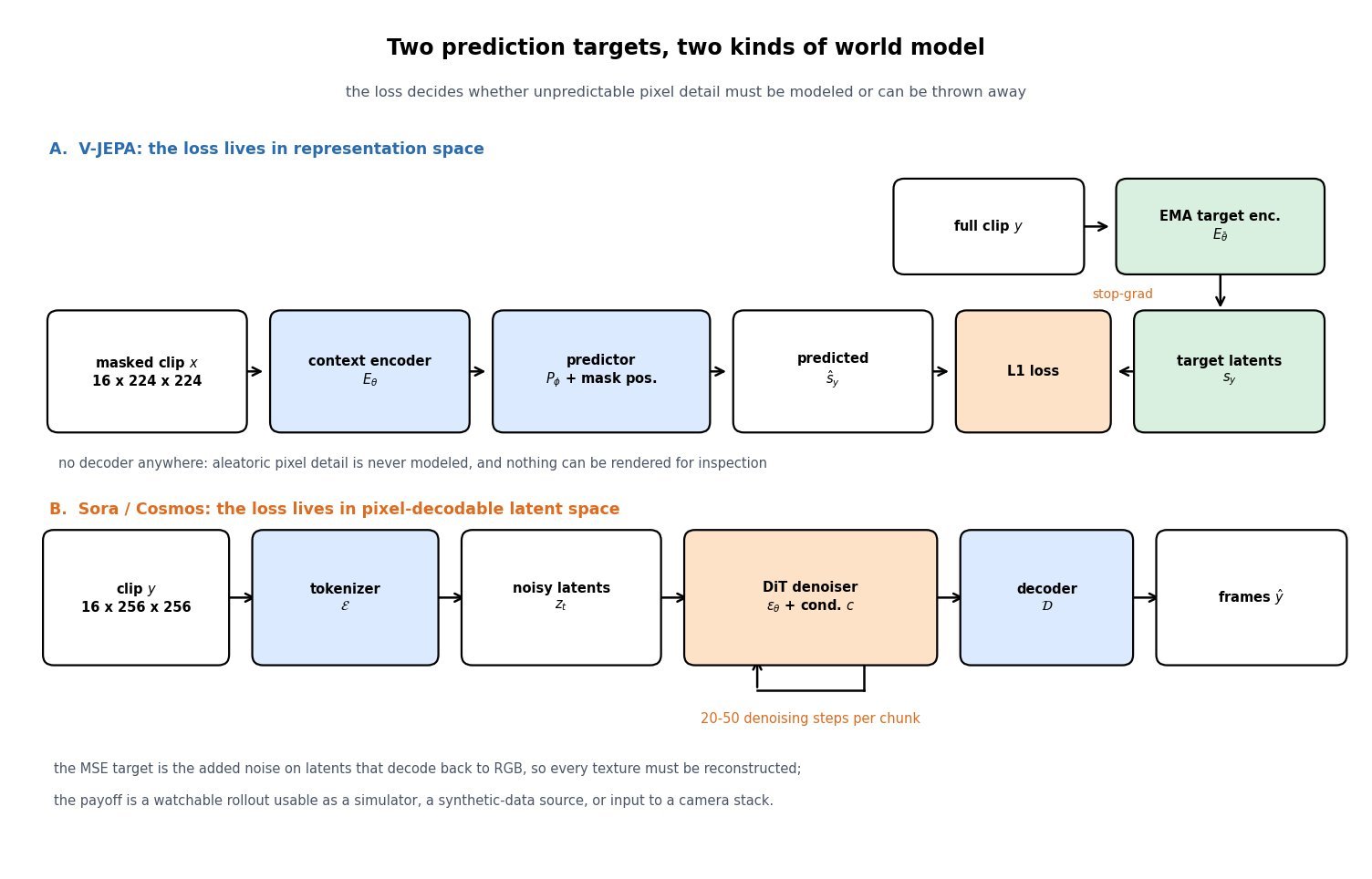
$\mathcal{L}_{\mathrm{gen}} = \mathbb{E}\left[\lVert \epsilon - \epsilon_{\theta}(z_t, t, c) \rVert_2^2\right]$
$a^{*} = \arg\min_{a} \lVert P_{\phi}(s_t, a) - s_g \rVert_1$

Where:

$x$ is the visible (context) part of a clip and $y$ the masked target region; $m$ carries the positional mask tokens telling the predictor where to predict.
$E_{\theta}$ is the online encoder, $E_{\bar{\theta}}$ the EMA target encoder, and $P_{\phi}$ the narrow predictor discarded after pretraining.
$\mathrm{sg}(\cdot)$ is the stop-gradient that blocks the trivial solution, and $\tau$ is the EMA momentum, typically ramped from about 0.998 toward 1.
$z_t$ is the noised tokenizer latent at diffusion step $t$ , $\epsilon$ the sampled Gaussian noise, $\epsilon_{\theta}$ the denoiser, and $c$ the conditioning (text, past frames, or actions).
$s_t$ is the current latent state, $a$ a candidate action sequence, and $s_g$ the goal embedding; the planner requires an initial condition $s_t = E_{\theta}(o_t)$ from the current observation.

Log-scale bar chart of forward passes per planning step for a 200-candidate 16-step CEM search: 3200 for a one-pass latent predictor, 12800 for a distilled four-step video diffusion model, and 96000 for a thirty-step video diffusion world model

Figure 2: For the same 200-candidate, 16-step CEM search, a single-pass latent predictor needs 3,200 network calls while a 30-step generative rollout needs 96,000, before the decoder is even invoked; this 30x gap is why planning loops favor latent prediction.

Property	V-JEPA (latent predictive)	Sora / Cosmos (generative world model)
Training target	Embeddings from an EMA copy of the encoder, L1 loss	Noise or next token on VAE latents that decode to RGB
Handles stochastic detail by	Dropping it from the representation	Sampling it, which costs capacity and steps
Can render a future	No decoder; futures exist only as vectors	Yes, watchable and consumable by any vision stack
Cost per rollout step	One predictor forward pass	Tens of denoiser passes plus a decode
Main pathology	Representation collapse and shortcut solutions under weak masking	Physically implausible but photoreal rollouts, plus error accumulation over long horizons
Natural deployment	Frozen backbone for recognition and anticipation; goal-conditioned planning	Synthetic data, neural simulators, scenario replay, content generation

August 17, 2026