
How do end-to-end autonomous driving architectures combine world model generation with trajectory scoring and cost function evaluation to select the safest driving path?
Answer
Competitive end-to-end stacks do not regress one trajectory and drive it. They propose many candidates, imagine the future under each one, and then take the argmax of an explicit cost, which turns planning into a ranking problem over a finite action set. The world model is what makes the ranking meaningful: it is an ego-conditioned forecaster that answers a counterfactual question, namely what the agents, the occupancy grid, or the camera views would look like if this particular trajectory were executed. The cost function then reads that imagined rollout and produces bounded sub-metrics for collision, drivable-area compliance, time-to-collision, comfort, and progress, which are combined so that hard safety terms multiply and soft preference terms are averaged. Because rolling out a simulator for thousands of candidates is far too slow at a 10 Hz replanning rate, production designs run the expensive scorer offline as a teacher and distill it into a small scoring head that evaluates the whole vocabulary in one batched forward pass.
(1) Proposal Set Instead Of Regression: a fixed trajectory vocabulary (8192 clustered 4-second trajectories in Hydra-MDP, 4096 in VADv2) or a small set of diffusion anchors preserves multi-modality and gives the cost function something concrete to compare.
(2) Ego-Conditioned World Model: the rollout must be conditioned on the candidate action, otherwise every candidate shares one predicted future and the scores carry no causal information about the ego’s own choice.
(3) Multiplicative Gates Plus Weighted Soft Terms: collision and off-road terms enter as multiplicative factors so a single violation zeroes the score, while time-to-collision, comfort, and progress enter as a weighted average that only re-ranks the survivors.
(4) Simulator As Teacher, Head As Student: a rule-based closed-loop metric computed with LQR tracking on a bicycle model labels every candidate offline, and a cross-attention scoring head learns those labels, converting a multi-second simulation into a millisecond-scale inference.
(5) Reactivity Decides Validity: non-reactive rollouts hold other agents on their logged paths, which systematically over-rewards cutting in and under-penalizes aggressive gap acceptance.
(6) Latency Sets The Design: a 4-second horizon at 10 Hz is 40 poses per candidate and the whole loop must close inside about 100 ms, which rules out per-candidate video generation online.
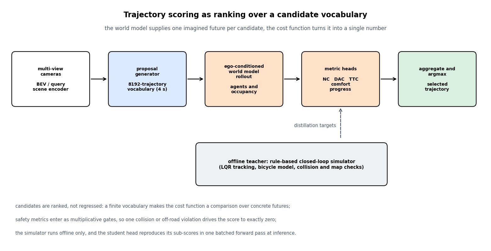
Figure 1: One scene encoder, many candidates, one score. The world model rollout is evaluated per candidate, and the metric heads are trained against an offline rule-based simulator, so the simulator’s judgement is available at inference without running it.
The world model shows up in three distinct roles, and confusing them is a common interview mistake. In the in-loop role, a generative model such as Drive-WM synthesizes multi-view future frames conditioned on each candidate and an image-space reward built from map and object cues picks the branch, which is expressive but so expensive that only a shallow tree of a few branches is affordable. In the representation role, future-occupancy or future-agent forecasting is an auxiliary head that shapes the BEV latent, so cost terms are computed on predicted geometry rather than pixels, which is the practical choice inside a 100 ms budget. In the offline role, high-fidelity generators supply rare scenarios and closed-loop training environments, so the cost function is validated against near-misses that almost never appear in logged data. Whatever the role, the failure mode is the same: if the rollout ignores that other agents respond to the ego, the cost function rewards trajectories that would have been vetoed by any reactive simulator.

Figure 2: Why the aggregation is multiplicative rather than additive. Candidates A and B are gated to exactly zero by collision and drivable-area violations no matter how much progress they buy, and only then do the soft terms separate the timid full stop from the trajectory that actually makes progress.
Mathematical Formulation:


Where:
 is the executed trajectory and the candidate vocabulary, typically a few thousand clustered 4-second trajectories sampled at 10 Hz.
- is the sensor history, the ego-conditioned world model, and the imagined future over horizon under that specific .
- extracts metric from the rollout and is its value, bounded to the unit interval so that scores are comparable across scenes.
- are the gate metrics (no at-fault collision, drivable-area compliance) whose product vetoes a candidate outright.
- are the weights of the soft metrics (time-to-collision, comfort, ego progress) aggregated by , which only re-ranks candidates that passed every gate.
 is the executed trajectory and
 the candidate vocabulary, typically a few thousand clustered 4-second trajectories sampled at 10 Hz.
 is the sensor history,
 the ego-conditioned world model, and
 the imagined future over horizon
 under that specific
 .
 extracts metric
 from the rollout and
 is its value, bounded to the unit interval so that scores are comparable across scenes.
 are the gate metrics (no at-fault collision, drivable-area compliance) whose product
 vetoes a candidate outright.
 are the weights of the soft metrics (time-to-collision, comfort, ego progress) aggregated by
 , which only re-ranks candidates that passed every gate.
NAVSIM PDM Score Instantiation:


Here NC and DAC are binary gates, while time-to-collision, comfort, and ego progress carry weights 5, 2, and 5. The weights are the policy: raising the progress weight produces a stack that squeezes through gaps, and raising comfort produces one that refuses to brake late. The distillation objective simply asks the student head to reproduce every teacher sub-metric per candidate.
Distillation And Latency Budget:


Figure 3: Representative per-candidate costs against the 100 ms replanning budget. A distilled scoring head is almost flat in the number of candidates because scoring is one batched forward pass, a rule-based simulator caps out near a hundred candidates, and a per-candidate video rollout blows the budget on its first branch.
| Property | Rule-based simulator in the loop | Generative world model in the loop | Distilled learned scorer |
|---|---|---|---|
| Proposal source | Centerline offsets crossed with target speeds, about 15 proposals | A shallow tree of a few branches per replan | Clustered vocabulary of 4096 to 8192 trajectories, or 20 diffusion anchors |
| How futures are obtained | Bicycle model plus LQR tracking with map and collision checks | Diffusion rollout of multi-view frames or occupancy conditioned on the action | No explicit rollout at inference, the head predicts each sub-metric directly |
| Agent reactivity | Configurable, IDM background traffic reacts to the ego | Learned and implicit, quality depends entirely on training data | Inherited from whatever the teacher assumed, usually non-reactive logs |
| Per-candidate cost | Sub-millisecond but CPU-bound and linear in candidates | Hundreds of milliseconds of GPU time per branch | Microseconds, batched inside one transformer forward pass |
| Dominant failure mode | Hand-written dynamics and a coarse proposal set miss creative maneuvers | Hallucinated geometry, action leakage, and unusable latency | Copies the teacher’s blind spots and can latch onto ego-status shortcuts |
Leave a Reply