
How does Principal Component Analysis (PCA) work, step by step?
Answer
PCA finds the orthogonal directions of maximum variance in centered data and projects the data onto the top  of them. Step by step: center each feature by subtracting its mean (and scale to unit variance when units differ); compute the covariance matrix; eigendecompose it, or equivalently run SVD on the data matrix, so eigenvectors become the principal directions and eigenvalues the variance each direction carries; keep the top eigenvectors and project every sample onto them. The result is a rotated coordinate system whose axes are uncorrelated and ordered by explanatory power, which is why the first few components often carry most of the variance.
(1) Variance as Information: each principal component is the direction of maximum residual variance, orthogonal to all previous ones, and its eigenvalue  is exactly the variance the data has along it.
(2) Explained-Variance Ratio Picks k: plot the cumulative share  and keep enough components to cover, say, 95% of total variance.
(3) Linear and Scale-Sensitive: PCA rotates but never unrolls, so curved manifolds need non-linear methods, and features with different units must be standardized first. Learned embeddings sidestep truncation differently: OpenAI’s text-embedding-3 models were trained with Matryoshka representation learning, so shortening a 3072-dimension vector to 256 still beats the older full-size ada-002, a property naive PCA truncation of a learned embedding cannot promise.
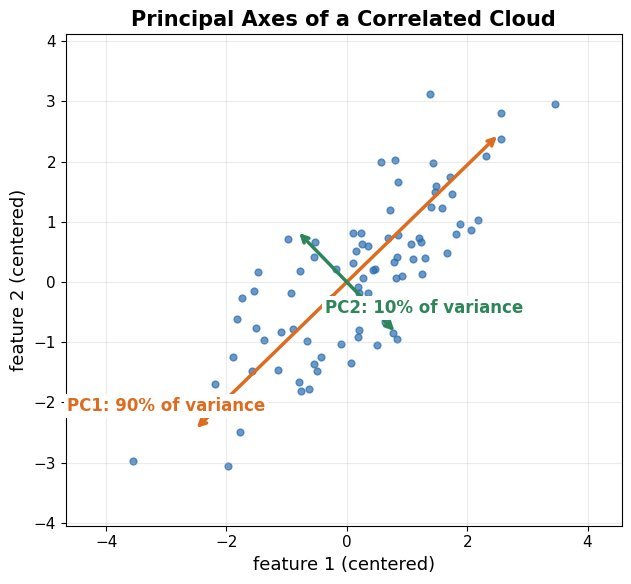
Figure 1: The two principal components of a 2D cloud: PC1 lies along the direction of maximum spread and carries the largest eigenvalue; PC2 is orthogonal to it and mops up the residual variance.
Mathematical Formulation:


Where:
 is the centered data matrix with samples and features; is its covariance matrix.
- are the eigenvector-eigenvalue pairs of , sorted by descending .
- stacks the top eigenvectors and is the -dimensional score vector of sample .
 are the eigenvector-eigenvalue pairs of
 stacks the top
 is the
 .

Figure 2: The scree plot: bars show the variance each component carries and the curve shows the cumulative share. Keeping components up to the 95% crossing is the standard rule for choosing .
Projection is lossy: the discarded components carry the remaining variance, so projecting back into the original space reconstructs the data only up to the kept subspace. In 2D this means every point collapses onto the PC1 line when only one component is kept, which is the geometric picture behind “95% of variance retained”.
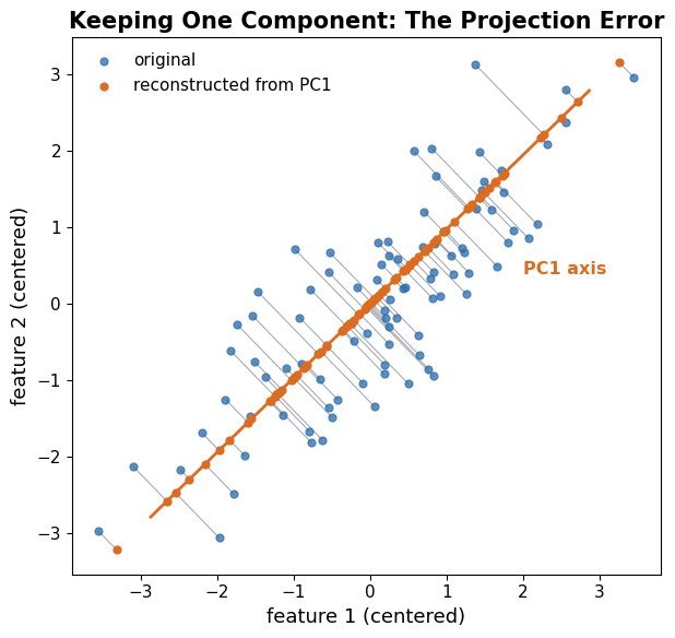
Figure 3: Reconstruction from one component: every point is replaced by its perpendicular projection onto the PC1 axis. The gray connectors are the reconstruction errors, whose mean squared length is exactly the discarded variance  (their sum is
 ).
| Feature | Eigendecomposition of Covariance | SVD of the Data Matrix |
|---|---|---|
| Input | The  matrix  | The centered  matrix  directly |
| Numerical Stability | Forming  squares the condition number | Stable: never materializes |
| Scalability | Fine for small  | Randomized SVD scales to huge  and |
| Practice | Textbook derivation | What libraries (scikit-learn) actually call |
Leave a Reply