How to choose the number of features in a random forest?
Answer
Select the number of features ( ) using rules of thumb (default heuristics), then tune via cross-validation or out-of-bag (OOB) error to find the best value for your specific dataset.
Default Heuristics:
Classification: 
Regression: 
Where: = total number of features, = number of features considered at each split.
Bias-Variance Trade-off:
(1) Smaller max_features will increase randomness, leading to less correlated trees (reducing variance) but potentially higher bias.
(2) Larger max_features will decrease randomness, leading to more correlated trees (increasing variance) but potentially lower bias.
Grid Search/Randomized Search:
This is the most robust method. Define a range of possible max_features values and use cross-validation to evaluate the model’s performance for each value.
Out-of-Bag (OOB) Error:
Random Forests can estimate the generalization error internally using OOB samples. You can monitor the OOB error as you vary max_features to find the optimal value.
The figure below shows the cross-validation accuracy curve when using different numbers of features.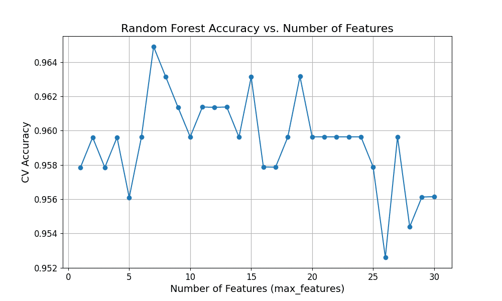

 = prediction of the b-th tree.
 = total number of trees.

 nearest neighbors. The majority votes for classification. Average of values for regression.

 is the set of points in cluster
  .
. is the centroid of cluster
  is a data point assigned to cluster

 is the data point.
 is the cluster center.
 represents the set of points assigned to cluster
  .
.

 is the predicted value for the query point.
 represents the target value of the i‑th nearest neighbor.
 nearest neighbors of a test point, using a chosen distance metric. It is intuitive and effective for small datasets, though less efficient on large-scale data.
 , it computes the distance to every training point (e.g., Euclidean distance).
 and
and  th features of the new and training points, respectively.
 is the number of features
 is the predicted class label for the query point.
 represents the set of all possible classes.
 is an indicator function, returning 1 if the neighbor’s class is
  , and 0 otherwise.
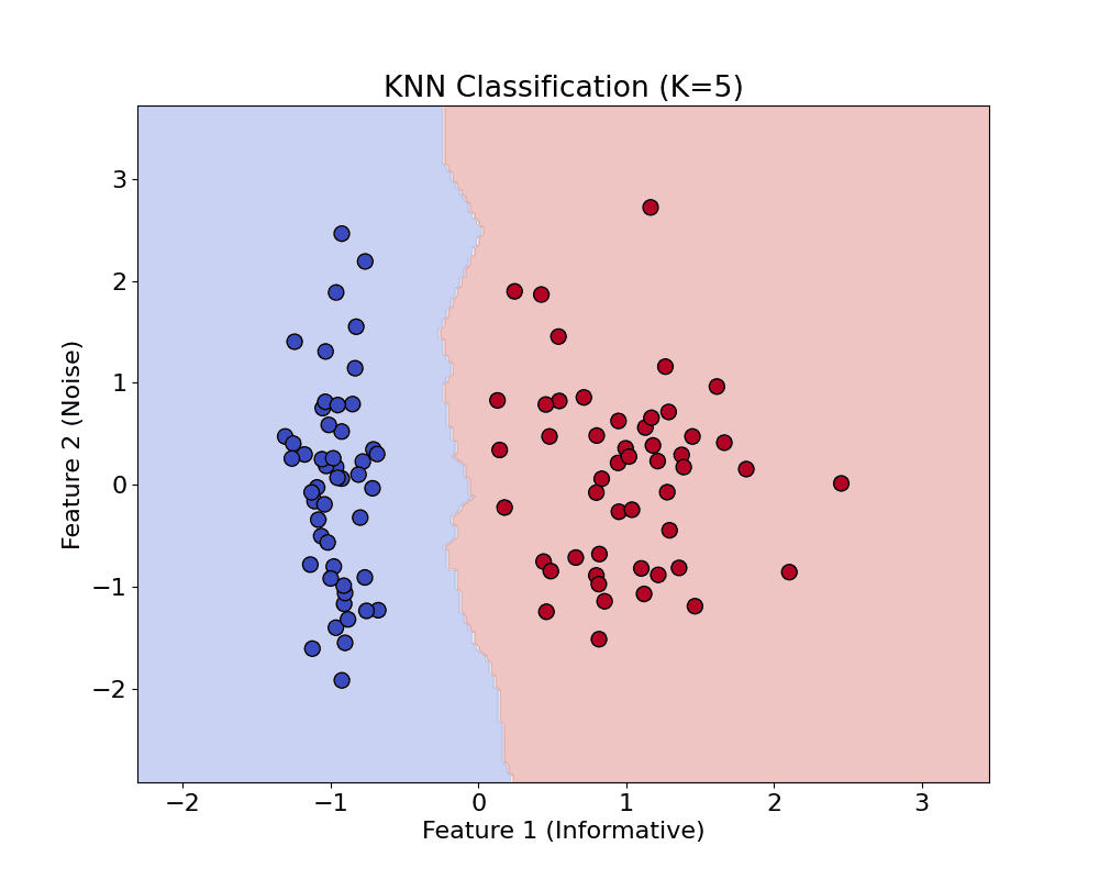

 is the true label,
 is the raw model output.
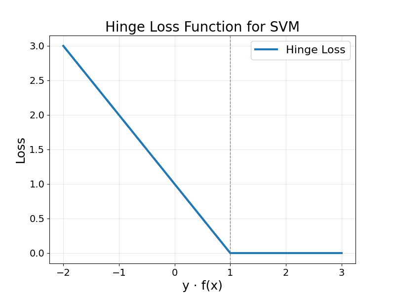
 , meaning the point is correctly classified with margin.
 , the point is either inside the margin or misclassified.
 is the weight vector.
 is the bias term.
 returns +1 if the argument is ≥ 0, and −1 otherwise.

 is the class label for the i-th data point.
 is the i-th feature vector.