Author: admin

  • DL0067 BERT VS GPT Pretraining

    How does BERT’s pre-training objective differ from GPT’s?

    Answer

    BERT is trained primarily with masked language modeling: selected input tokens are corrupted, and a bidirectional encoder predicts the original tokens from visible context on both sides. GPT uses causal language modeling: a decoder predicts each next token using only earlier tokens, enforced by a triangular attention mask. MLM supplies loss only at selected positions and creates a corruption mismatch between pre-training and ordinary inputs, whereas causal modeling supplies a target at nearly every position and matches left-to-right generation. Original BERT also used next sentence prediction, while standard GPT pre-training relies on the autoregressive token objective rather than NSP.

    Side-by-side BERT masked-language-modeling and GPT causal-language-modeling pre-training objectives.

    Figure 1: BERT reconstructs selected corrupted tokens from two-sided context, while GPT predicts the next token at every step from a left-only prefix.

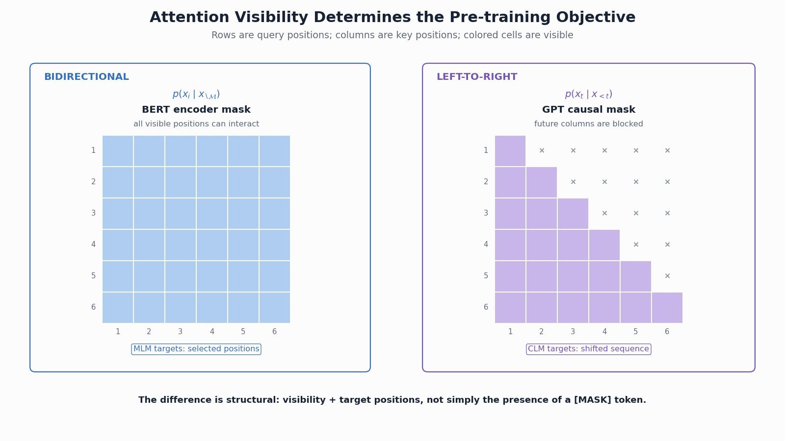
    (1) Context Visibility: BERT’s visible tokens attend bidirectionally; GPT position t cannot attend to positions later than t.
    (2) Prediction Targets: BERT reconstructs a selected masked subset, while GPT shifts the sequence and predicts the next token at each usable position.
    (3) Downstream Bias: BERT naturally supports full-context understanding, whereas GPT’s objective directly trains open-ended autoregressive generation; either family can be adapted beyond that bias.

    Mathematical Formulation:
    \mathcal{L}_{\mathrm{BERT}}=-\sum_{i\in\mathcal{M}}\log p(x_i\mid x_{\setminus\mathcal{M}})
    \mathcal{L}_{\mathrm{GPT}}=-\sum_{t=1}^{T}\log p(x_t\mid x_{1:t-1})

    Where:

    • \mathcal{L}_{\mathrm{BERT}} and \mathcal{L}_{\mathrm{GPT}} are the masked and causal language-modeling losses.
    • \mathcal{M} is BERT’s selected target set and i\in\mathcal{M} indexes one target token x_i.
    • x_{\setminus\mathcal{M}} denotes BERT’s visible corrupted context outside the selected targets, and p(x_i\mid x_{\setminus\mathcal{M}}) is the reconstruction probability.
    • t\in\{1,\ldots,T\} indexes a GPT target position, T is sequence length, and x_{1:t-1} is the preceding token prefix.
    • p(x_t\mid x_{1:t-1}) is the next-token probability and \log converts each probability into a log-likelihood term.
    BERT bidirectional and GPT causal attention matrices with their respective training target positions.

    Figure 2: Attention visibility explains the objective difference: BERT uses a full visible-context matrix, while GPT uses a lower-triangular causal matrix.

    Login to view more content
  • DL0066 BERT

    What is BERT and how is it used in NLP tasks?

    Answer

    BERT is a Transformer encoder pretrained to build bidirectional contextual representations of text. Its input combines token, segment, and positional embeddings, and every encoder layer lets each unmasked token attend to context on both sides. Original BERT is pretrained with masked language modeling and next sentence prediction, then adapted by adding a small task head and fine-tuning the whole model or using its representations. The [CLS] output supports sequence-level tasks, token outputs support tagging, and paired start/end scores support extractive question answering.

    BERT input embeddings and bidirectional Transformer encoder producing contextual token representations.

    Figure 1: BERT combines token, segment, and position embeddings, processes them with bidirectional encoder layers, and exposes contextual outputs.

    (1) Bidirectional Encoder: Unlike a causal decoder, BERT‘s self-attention normally uses both left and right context for every visible input token.
    (2) Pre-Training: Original BERT predicts selected masked tokens and also trains an NSP classifier; later BERT-family models often modify or remove NSP.
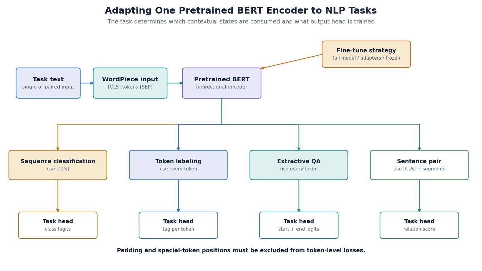
    (3) Task Adaptation: A lightweight output head maps contextual states to sequence labels, token labels, sentence-pair scores, or answer spans.

    BERT fine-tuning flowchart for classification, token labeling, question answering, and sentence pairs.

    Figure 2: The same pretrained encoder can be adapted with small heads that consume either [CLS], every token state, or start/end span scores.

    Mathematical Formulation:
    H=\mathrm{Encoder}(E_{\mathrm{token}}+E_{\mathrm{segment}}+E_{\mathrm{position}})
    \mathcal{L}_{\mathrm{MLM}}=-\sum_{i\in\mathcal{M}}\log p(x_i\mid x_{\setminus\mathcal{M}})

    Where:

    • E_{\mathrm{token}}, E_{\mathrm{segment}}, and E_{\mathrm{position}} are token, segment, and positional embedding matrices for the input sequence.
    • \mathrm{Encoder} is the bidirectional Transformer stack and H contains one contextual vector per input position.
    • \mathcal{L}_{\mathrm{MLM}} is masked-language-modeling loss and \mathcal{M} is the selected set of prediction positions.
    • i\in\mathcal{M} indexes one selected target, x_i is its original token, and x_{\setminus\mathcal{M}} denotes the visible corrupted context outside the selected targets.
    • p(x_i\mid x_{\setminus\mathcal{M}}) is the model probability assigned to the original target token given visible context.

    Login to view more content
  • DL0065 Group Normalization

    What is Group Normalization?

    Answer

    Group Normalization normalizes each sample independently by dividing its channels into groups and computing a mean and variance over the channels and spatial positions within each group. The normalized activations then receive learned per-channel scale and shift parameters. Because its statistics do not depend on other examples, GroupNorm behaves consistently with very small or variable batch sizes and uses the same computation during training and inference. The group count must be compatible with the channel count, and its inductive bias can be less suitable than BatchNorm when large, stable batches provide useful batch statistics.

    Group Normalization mechanism partitioning channels and normalizing each sample group.

    Figure 1: A convolutional tensor is split into channel groups; each sample-group gets independent statistics before per-channel affine scaling.

    (1) Per-Sample Statistics: Each example has its own group means and variances, so no running batch averages are required.
    (2) Channel Grouping: For C channels and G groups, each group normalizes (C/G)\times H\times W values; channels within a group share statistics.
    (3) Boundary Cases: G=1 normalizes all channels and spatial positions together, while G=C gives one channel per group and resembles InstanceNorm.

    Comparison of Batch, Layer, Instance, and Group Normalization reduction dimensions.

    Figure 2: Normalization families differ mainly in which batch, channel, and spatial axes share statistics and whether inference needs running estimates.

    Mathematical Formulation:
    \mu_{n,g}=\frac{1}{m}\sum_{i\in S_{n,g}}x_i
    \sigma^2_{n,g}=\frac{1}{m}\sum_{i\in S_{n,g}}(x_i-\mu_{n,g})^2
    y_{n,c,h,w}=\gamma_c\frac{x_{n,c,h,w}-\mu_{n,g(c)}}{\sqrt{\sigma^2_{n,g(c)}+\epsilon}}+\beta_c

    Where:

    • n indexes samples, g indexes channel groups, and c,h,w index channel and spatial position.
    • S_{n,g} is the set of activations in group g of sample n; i indexes elements in that set.
    • m=(C/G)HW is the number of normalized values when C channels are divided into G groups over height H and width W.
    • \mu_{n,g} and \sigma^2_{n,g} are the group mean and variance; x and y are input and normalized output activations.
    • g(c) maps channel c to its group, \gamma_c,\beta_c are learned per-channel scale and shift, and \epsilon stabilizes division.

    Login to view more content
  • DL0064 CNNs Object Detection and Segmentation

    What is the role of CNNs in object detection and segmentation?

    Answer

    In object detection and segmentation, a CNN commonly acts as a spatial feature extractor that converts pixels into a hierarchy of increasingly semantic feature maps. Detection heads use those features to classify objects and localize bounding boxes, while segmentation heads upsample and fuse spatial detail to predict per-pixel classes or instance-specific masks. Multiscale features are important because small objects need high-resolution maps and large objects benefit from deeper receptive fields. CNNs are therefore the backbone and often part of the head, but proposal logic, feature pyramids, decoders, and task losses complete the system; modern vision Transformers can also replace or complement the CNN backbone.

    CNN multiscale backbone branching into object detection and image segmentation heads.

    Figure 1: A shared convolutional feature hierarchy supports two different outputs: sparse boxes and classes versus dense semantic or instance masks.

    (1) Shared Backbone: Convolutions provide translation-equivariant local processing and reusable feature maps at several strides.
    (2) Detection Role: One-stage or region-based heads turn features into class scores and box coordinates, often using multiscale pyramids.
    (3) Segmentation Role: Dense decoders combine semantic context with fine spatial detail for semantic labels, instance masks, or panoptic outputs.

    Flowchart comparing CNN processing for detection, semantic segmentation, and instance segmentation.

    Figure 2: Task-specific paths after the backbone show what each head must predict and how its output aligns with the input image.

    Mathematical Formulation:
    F_l=\mathrm{CNN}_l(I)
    (\hat b,\hat p)=H_{\mathrm{det}}(\{F_l\})
    \hat M=H_{\mathrm{seg}}(\{F_l\})
    \hat M\in\mathbb{R}^{H\times W\times K}

    Where:

    • I is the input image and F_l is the backbone feature map produced by stage l.
    • \{F_l\} is the multiscale feature set supplied to task heads.
    • H_{\mathrm{det}} is the detection head, with \hat b denoting predicted boxes and \hat p predicted class probabilities.
    • H_{\mathrm{seg}} is the segmentation head and \hat M is its dense output mask or logit tensor.
    • H and W are output height and width, while K is the number of semantic classes or mask channels.

    Login to view more content
  • DL0063 Transformer Variable Length Sequences

    How does the Transformer handle variable-length sequences?

    Answer

    A Transformer can process different sequence lengths because self-attention is defined over whatever number of tokens is supplied, up to the model’s context limit. For efficient batching, implementations usually pad sequences to a common length or group examples of similar lengths, then apply a padding mask so valid queries cannot attend to padded keys and values. Decoder-style models also add a causal mask that blocks future positions, while positional encodings identify token order within each sequence. Padded query outputs and losses must be ignored, and computation still scales with the padded batch length rather than only the number of valid tokens.

    (1) Batch Construction: Sequences are dynamically padded to the longest item in a batch, bucketed by length, or packed by specialized kernels to reduce wasted work.
    (2) Attention Masking: A key-padding mask removes padded keys and values from attention; causal models combine it with a triangular future mask.
    (3) Length Boundary: Variable length does not mean unlimited length: positional support, memory, and the configured context window impose a maximum.

    Variable-length token sequences padded into one batch with key-padding and causal attention masks.

    Figure 1: Unequal token sequences become a rectangular batch; masking separates valid context, padding, and future positions.

    Mathematical Formulation:
    \mathrm{Attention}(Q,K,V)=\mathrm{softmax}\!\left(\frac{QK^\top}{\sqrt{d_k}}+M_{\mathrm{pad}}+M_{\mathrm{causal}}\right)V
    M_{ij}\in\{0,-\infty\}

    Where:

    • Q, K, and V are query, key, and value matrices, and d_k is the key width used for score scaling.
    • M_{\mathrm{pad}} assigns -\infty to padded key positions so their softmax probabilities become zero.
    • M_{\mathrm{causal}} assigns -\infty when key index j is later than query index i; encoder-only models normally omit this mask.
    • M_{ij} denotes one combined mask entry and is either 0 for an allowed connection or -\infty for a blocked connection.
    • B is batch size and L_{max} is padded sequence length, giving a dense token tensor of shape B\times L_{max}.
    Transformer variable-length processing flowchart from tokenization through masks and output cleanup.

    Figure 2: A practical variable-length pipeline: tokenize, bucket or pad, build masks, run attention, then ignore padded outputs or continue autoregressive generation.


    Login to view more content
  • DL0062 LSTM

    What is an LSTM (Long Short-Term Memory) network? How does it address vanishing gradients?

    Answer

    A Long Short-Term Memory network is a gated recurrent neural network designed to carry useful information across many sequence steps. Each cell maintains a cell state and uses forget, input, and output gates to control what is retained, written, and exposed. Its additive cell-state update creates a shorter gradient path than repeatedly multiplying through a vanilla RNN’s nonlinear state transition, so gradients can remain useful when forget gates stay near one. LSTMs mitigate vanishing gradients rather than eliminating them: saturated gates, long products of forget factors, and poor optimization can still weaken learning.

    LSTM cell architecture showing forget, input, candidate, and output gates around the cell-state path.

    Figure 1: One LSTM timestep: gated reads and writes surround an additive cell-state highway, while the output gate produces the hidden state.

    (1) Two Recurrent States: The cell state c_t is the long-term memory path, while the hidden state h_t is the exposed representation used by the next step and downstream layers.
    (2) Gated Update: The forget gate scales old memory, the input gate controls a candidate update, and the output gate selects how much of the updated memory becomes visible.
    (3) Gradient Preservation: The derivative along the direct cell-state path contains products of forget gates instead of repeated full recurrent Jacobians; values near one preserve gradient flow.

    Mathematical Formulation:
    f_t=\sigma\!\left(W_f[x_t,h_{t-1}]+b_f\right)
    i_t=\sigma\!\left(W_i[x_t,h_{t-1}]+b_i\right)
    \tilde c_t=\tanh\!\left(W_c[x_t,h_{t-1}]+b_c\right)
    c_t=f_t\odot c_{t-1}+i_t\odot\tilde c_t
    o_t=\sigma\!\left(W_o[x_t,h_{t-1}]+b_o\right)
    h_t=o_t\odot\tanh(c_t)

    Where:

    • t is the timestep; x_t is the current input, and h_{t-1},c_{t-1} are the previous hidden and cell states.
    • f_t,i_t,o_t\in(0,1) are element-wise forget, input, and output gates; \tilde c_t is the candidate cell update.
    • c_t is the updated long-term cell state and h_t is the exposed hidden state.
    • W_f,W_i,W_c,W_o and b_f,b_i,b_c,b_o are learned affine parameters; [x_t,h_{t-1}] denotes concatenation.
    • \sigma is sigmoid, \tanh is hyperbolic tangent, and \odot is element-wise multiplication; the direct derivative includes \partial c_t/\partial c_{t-1}=f_t.
    Comparison of gradient propagation through a vanilla recurrent network and an LSTM cell-state path.

    Figure 2: Why LSTMs mitigate vanishing gradients: a vanilla RNN repeatedly multiplies full nonlinear Jacobians, whereas the LSTM provides a gated direct memory path.


    Login to view more content
  • DL0061 Channel and Spatial Attention

    Explain channel attention and spatial attention in CNNs. What information does each mechanism model?

    Answer

    Channel attention learns which feature channels are important, answering what semantic responses should be emphasized. It compresses spatial dimensions into channel descriptors, transforms them with a small gating network, and multiplies the resulting weights into the feature tensor. Spatial attention learns where informative regions occur by compressing or projecting the channel dimension and producing an H\times W mask. Modules such as SE use channel attention, while CBAM applies channel attention followed by spatial attention to refine both feature type and location.
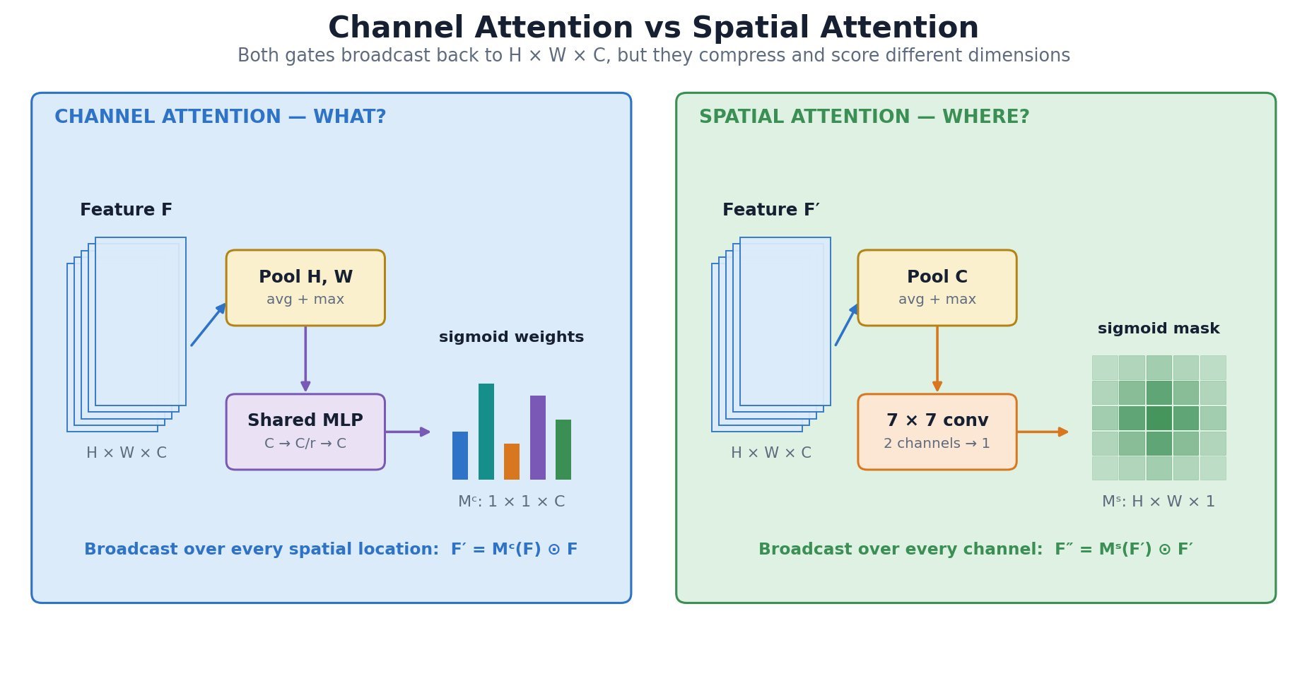
    Channel attention and spatial attention mechanisms with tensor reductions and broadcast multiplication.

    Figure 1: Parallel tensor-shape explanation of what channel attention selects and where spatial attention focuses.

    (1) Channel Gate: Global pooling summarizes each channel; an MLP or 1D convolution captures inter-channel dependence and outputs C multiplicative weights.
    (2) Spatial Gate: Average/max pooling or learned projection across channels produces spatial descriptors that a convolution maps to one H\times W attention mask.
    (3) Residual Placement: Attention usually modulates an existing feature tensor and is often inserted inside a residual block; sigmoid gates reweight rather than replace the underlying features.

    Sequential CBAM channel-then-spatial attention flowchart.

    Figure 2: CBAM data flow from input feature through channel gating, spatial gating, residual refinement, and output.

    Mathematical Formulation:
    M_c(F)=\sigma\!\left(\mathrm{MLP}(\mathrm{AvgPool}_{hw}(F))+\mathrm{MLP}(\mathrm{MaxPool}_{hw}(F))\right)
    M_s(F)=\sigma\!\left(f^{7\times7}([\mathrm{AvgPool}_{c}(F);\mathrm{MaxPool}_{c}(F)])\right)

    Where:

    • F\in\mathbb{R}^{H\times W\times C} is the input feature map with height H, width W, and C channels.
    • M_c(F)\in\mathbb{R}^{1\times1\times C} is the channel mask; spatial average/max pooling and the shared \mathrm{MLP} produce channel logits.
    • M_s(F)\in\mathbb{R}^{H\times W\times1} is the spatial mask; channel pooling outputs are concatenated by [\,;\,] and filtered by f^{7\times7}.
    • \sigma is the sigmoid function; M_c broadcasts over H,W, while M_s broadcasts over C.

    Login to view more content
  • DL0060 Depthwise Separable Convolution

    What is depthwise separable convolution, and where is it commonly used?

    Answer

    Depthwise separable convolution factorizes a standard convolution into a depthwise spatial operation and a pointwise channel-mixing operation. The depthwise stage applies one k\times k filter per input channel, so it learns spatial patterns independently; the 1\times1 pointwise stage combines those channel responses into new output channels. This factorization can reduce multiply-accumulates and parameters by almost the kernel area when channel counts are large. It is common in MobileNet, Xception, EfficientNet-style mobile blocks, and edge models where latency, power, and model size matter.
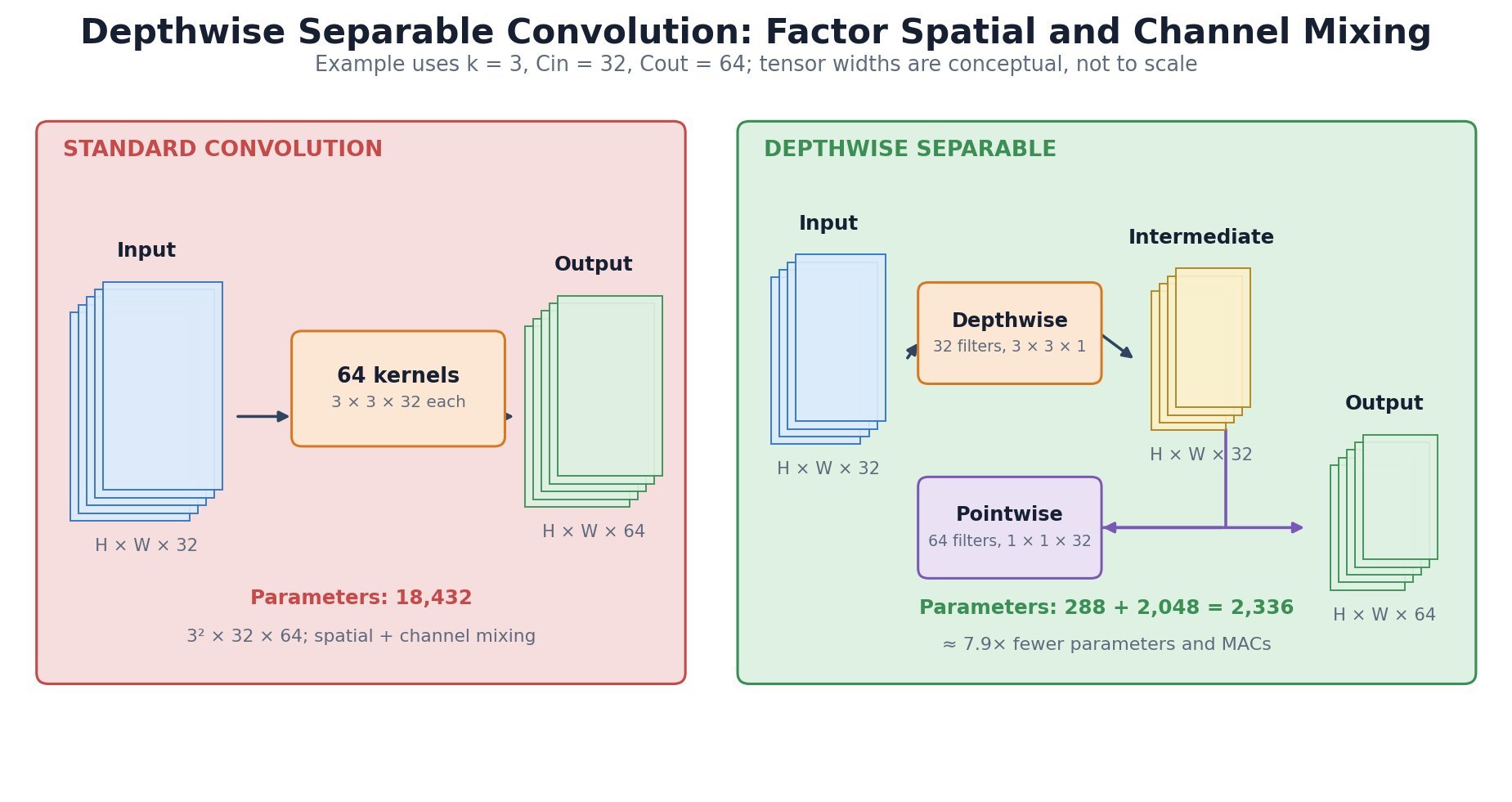
    Standard convolution compared with depthwise and pointwise factorization.

    Figure 1: Tensor-level view of spatial filtering per channel followed by 1×1 channel mixing, with parameters and MACs.

    (1) Depthwise Stage: With depth multiplier one, C_{in} independent k\times k filters produce C_{in} spatially filtered maps and do not mix channels.
    (2) Pointwise Stage: A 1\times1 convolution applies a learned C_{in}\times C_{out} channel transformation independently at every spatial position.
    (3) Real Hardware: Lower arithmetic cost does not guarantee proportional speedup because memory traffic, kernel launch overhead, vectorization, and accelerator support can dominate.

    Decision flowchart for choosing standard, grouped, or depthwise separable convolution.

    Figure 2: Architecture decision based on efficiency target, channel interaction, hardware kernels, and measured latency.

    Mathematical Formulation:
    \mathrm{MACs}_{std}=HWk^2C_{in}C_{out}
    \mathrm{MACs}_{sep}=HW\left(k^2C_{in}+C_{in}C_{out}\right)
    \frac{\mathrm{MACs}_{sep}}{\mathrm{MACs}_{std}}=\frac{1}{C_{out}}+\frac{1}{k^2}

    Where:

    • \mathrm{MACs}_{std} and \mathrm{MACs}_{sep} count multiply-accumulates for standard and depthwise-separable convolution.
    • H and W are output height and width, and k is the square spatial-kernel width.
    • C_{in} and C_{out} are input and output channel counts; the formula assumes depth multiplier 1.
    • For k=3 and large C_{out}, the ratio approaches 1/9.

    Login to view more content
  • DL0059 Transposed Convolution

    What is a transposed convolution (sometimes called deconvolution), and when is it used?

    Answer

    A transposed convolution is a learnable linear operator whose matrix is the transpose of the matrix representing a corresponding forward convolution. Operationally, each input value scatters a scaled kernel into an output grid, with stride controlling the spacing and overlapping contributions summed. It can increase spatial resolution, but it is not a mathematical inverse and does not recover information destroyed by downsampling. It is commonly used in semantic-segmentation decoders, generative models, learned reconstruction, and other architectures that map low-resolution features to higher-resolution outputs.

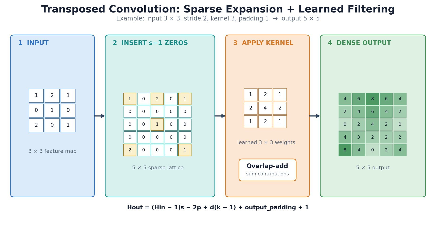
    Transposed convolution shown as zero insertion, kernel application, and overlap summation.

    Figure 1: A stride-2 transposed convolution decomposed into sparse expansion and learned filtering, including output-shape arithmetic.

    (1) Learned Upsampling: Unlike fixed nearest-neighbor or bilinear interpolation, the layer learns how feature values contribute to surrounding output positions.
    (2) Output Geometry: Kernel size, stride, padding, dilation, and output padding jointly determine the output shape; output padding resolves shape ambiguity but does not add zero-valued borders.
    (3) Artifact Risk: Uneven overlap occurs when the kernel size is not divisible by stride and can produce checkerboard artifacts, especially in image generators.

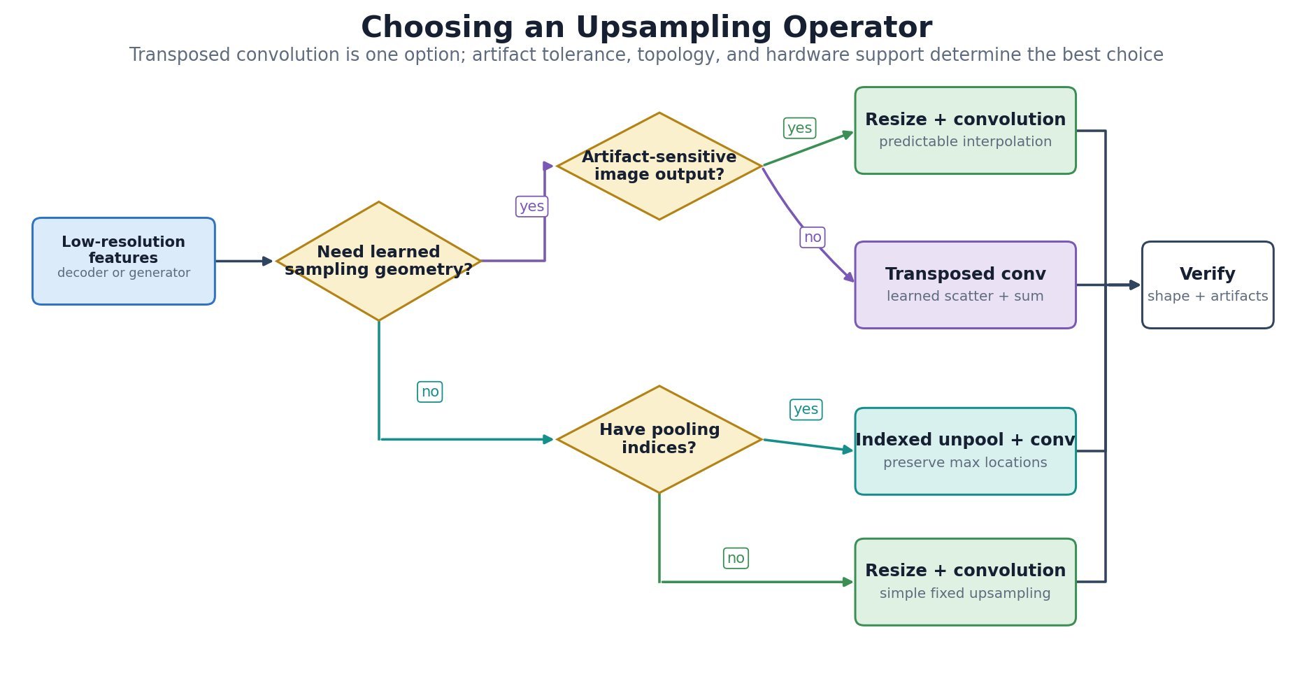
    Upsampling-method decision flowchart comparing transposed convolution, resize-convolution, and unpooling.

    Figure 2: Selection guide based on learned reconstruction, artifact sensitivity, pooling indices, and deployment constraints.

    Mathematical Formulation:
    H_{out}=(H_{in}-1)s-2p+d(k-1)+p_{out}+1

    Where:

    • H_{in} and H_{out} are the input and output sizes along one spatial axis.
    • s is stride, p is padding, d is dilation, and k is kernel size.
    • p_{out} is output padding used to choose among otherwise ambiguous valid output sizes; it does not append learned pixels.
    • The formula applies independently to width and, for 3D layers, depth by replacing H with the corresponding axis size.

    Login to view more content
  • DL0058 Feature Pyramid Network

    What is a pyramid network in the context of CNNs, and why is it useful for dense prediction?

    Answer

    A feature pyramid network (FPN) builds a hierarchy of semantically strong feature maps at multiple spatial resolutions. A bottom-up backbone produces progressively smaller maps with richer semantics; a top-down pathway upsamples deep features and merges them with same-resolution lateral projections from earlier stages. The resulting P_2\text{--}P_5 maps combine localization detail with high-level context. Detection, instance segmentation, and keypoint heads can then select a pyramid level appropriate to each object or region scale.

    Feature Pyramid Network architecture with bottom-up, lateral, and top-down paths.

    Figure 1: FPN construction showing tensor resolution, lateral 1×1 projection, top-down upsampling, fusion, and 3×3 smoothing.

    (1) Bottom-up Hierarchy: Backbone stages C_2\text{--}C_5 reduce spatial resolution while increasing receptive field and semantic abstraction.
    (2) Top-down Fusion: Nearest-neighbor upsampling and 1×1 lateral projections align channel widths before element-wise addition; a 3×3 convolution commonly smooths each merged map.
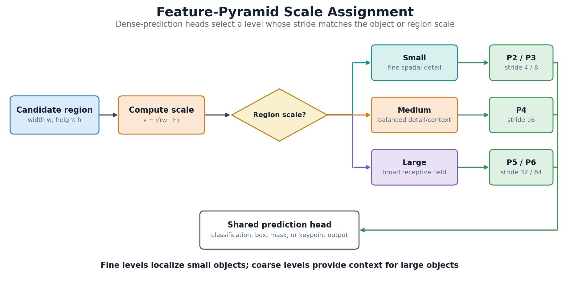
    (3) Scale Assignment: Small objects use high-resolution levels such as P_2 or P_3, while large objects use coarser levels such as P_4 or P_5.

    Feature pyramid scale-selection flowchart for small, medium, and large objects.

    Figure 2: How object size directs prediction heads toward fine, medium, or coarse pyramid levels.

    Mathematical Formulation:
    P_l=\mathrm{Conv}_{3\times3}\!\left(\mathrm{Conv}_{1\times1}(C_l)+\mathrm{Up}_2(P_{l+1})\right)
    k=\left\lfloor k_0+\log_2\!\left(\frac{\sqrt{wh}}{224}\right)\right\rfloor

    Where:

    • C_l is the bottom-up backbone feature and P_l is the fused pyramid output at level l.
    • \mathrm{Conv}_{1\times1} aligns channel width, \mathrm{Up}_2 doubles spatial resolution, and \mathrm{Conv}_{3\times3} smooths the merged feature.
    • k is the assigned pyramid level, k_0 is the reference level, and w,h are the region width and height.
    • 224 is the canonical reference scale and \lfloor\cdot\rfloor maps the continuous log-scale value to a discrete level.

    Login to view more content