
How does a GRU differ from an LSTM, and when would you prefer one over the other?
Answer
Both are gated recurrent cells that replace the vanilla RNN’s repeated multiplication by an additive state update, which is what keeps gradients alive across long sequences. The LSTM carries two state tensors (the cell state  and the hidden state
 ) and three gates: forget, input, and output. The GRU is a leaner reparameterization that keeps one state: it merges forget and input into a single update gate
 whose two branches are tied as and
 , deletes the output gate so the full state is exposed to the next layer, and adds a reset gate
 that suppresses the previous state inside the candidate. The practical consequence is three weight blocks instead of four, so roughly 25% fewer recurrent parameters and matmuls per step, plus one less tensor to carry and initialize. Accuracy is usually close (Chung et al. 2014; Greff et al. 2017), so the choice is driven by data size, latency, and whether the task needs the LSTM’s unbounded memory.
(1) Gate Inventory: LSTM has forget, input, and output gates; the GRU has update and reset only, because tying the write and erase decisions into and removes one gate and dropping the output gate removes another.
(2) One State vs Two: the LSTM’s protected cell state is never squashed on the recurrent path and is only revealed through the output gate, while the GRU’s single is both the memory and the emitted representation.
(3) Parameter and Compute Ratio: with input width  and hidden width
 , the GRU costs exactly
 of the LSTM’s recurrent parameters and per-step FLOPs, which matters most when the recurrent stack dominates the model.
(4) Expressivity Gap: at finite precision, the LSTM’s additive, unsquashed cell state can implement a genuine counter, whereas the GRU’s convex-combination update keeps the state inside  and can only approximate counting (Weiss et al. 2018).
(5) How to Choose: prefer the GRU for small or medium datasets, short-to-medium sequences, and tight latency or memory budgets; prefer the LSTM for long sequences, large corpora, and tasks that need precise long-horizon bookkeeping such as language modeling.

Figure 1: The LSTM keeps a separate cell-state track written by forget and input gates and read out through an output gate; the GRU folds everything onto one hidden-state track, where the update gate supplies both mixing weights and the reset gate only conditions the candidate.
Mathematical Formulation:


Where:
 is the hidden state emitted at step and the LSTM’s internal cell state; both start from zero at .
- is the input at step , with its width and the hidden width.
- are the LSTM forget, input, and output gates and its candidate, each of the form (with for the candidate).
- and are the GRU update and reset gates, both sigmoid, and is its candidate state.
- is the elementwise product, the logistic sigmoid mapping to , and the input, recurrent, and bias parameters of one gate block.
- counts recurrent-cell parameters only, so the ratio holds for any and .
 and
 .
 is the input at step
 are the LSTM forget, input, and output gates and
 its candidate, each of the form
 (with
 for the candidate).
 is its candidate state.
 is the elementwise product,
 the logistic sigmoid mapping to
 , and
 the input, recurrent, and bias parameters of one gate block.
 counts recurrent-cell parameters only, so the ratio
 holds for any
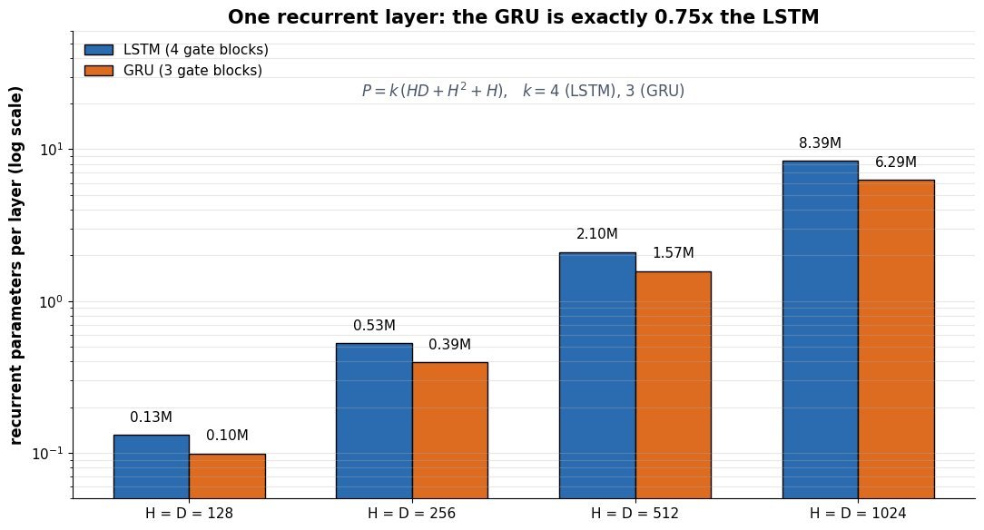
Figure 2: Recurrent parameters per layer with  : three gate blocks instead of four give the GRU exactly 0.75x the LSTM count at every width, so at
 one layer holds 1.57M against 2.10M.
| Property | GRU | LSTM |
|---|---|---|
| Gates | 2: update, reset | 3: forget, input, output |
| State carried | Hidden state only | Hidden state plus cell state |
| Weight blocks | 3 | 4 |
| Params at D = H = 512 | 1.57M | 2.10M |
| Memory exposure | Whole state is exposed downstream | Output gate filters what leaves the cell |
| Unbounded counting | No: state stays bounded by the convex update | Yes: additive, unsquashed cell state |
| Where it tends to win | Small data, short sequences, tight latency | Long sequences, large corpora, language modeling |
Leave a Reply