Category: Medium

DL0200 BERT GPU Underutilization

What can cause a BERT-based model to struggle with GPU underutilization, how do you detect CPU-side preprocessing bottlenecks, and what optimizations (pinned memory, ONNX export, TensorRT, INT8 quantization) would you recommend?

Answer

A BERT forward pass at batch 32 and sequence length 128 is a few milliseconds of dense GEMM work, so the GPU is almost never the slow part of a badly performing BERT service. Underutilization comes from three separable causes: the host-side pipeline (Python tokenization, collation, and synchronous host-to-device copies that block the training or serving loop), wasted GPU work (padding every request to max_length, batch size 1 traffic, or fragmented small kernels whose launch overhead exceeds their compute), and framework overhead (eager-mode PyTorch dispatching hundreds of tiny kernels per layer instead of fused ones). Detection is a matter of separating those causes rather than staring at the single nvidia-smi utilization number, which reports only whether any kernel was resident during a sampling window and happily shows 90% while the SMs are mostly idle. The fix ladder is ordered by cost: first hide the host work with fast tokenizers, multiple dataloader workers, pinned memory plus non_blocking copies and prefetch; then remove padding waste with length bucketing and dynamic batching; then export to ONNX for graph fusion and constant folding; then build a TensorRT engine in FP16; and only last apply INT8 post-training quantization, which is the only step in the list that can change your accuracy.

(1) Host-Bound Pipeline: a Python BertTokenizer plus per-batch collation can cost 15-25 ms while the forward pass costs 6 ms, so a serial loop pins utilization near 25% no matter how fast the GPU is.
(2) Synchronous Copies: a transfer from pageable host memory cannot be overlapped with compute, because the driver must stage it through an internal pinned buffer; pinned memory plus non_blocking=True is what makes DMA overlap legal.
(3) Padding Waste: attention cost scales as $O(L^2)$ , so padding a batch whose mean length is 27 tokens out to 128 burns roughly 79% of the tokens on [PAD], which looks like high utilization and low throughput.
(4) Kernel Launch Overhead: eager BERT-base issues on the order of a thousand kernels per forward pass; at batch 1 the launch and layout overhead, not the math, sets latency.
(5) Detection By Elimination: loop over one cached pre-tokenized tensor. If throughput jumps, the bottleneck was host-side; if it does not, profile kernels with Nsight Systems and look at gaps between them.
(6) Optimize In Cost Order: dataloader and padding fixes are free and safe, ONNX and TensorRT FP16 are numerically near-lossless, and INT8 is the only step that requires a calibration set and an accuracy regression gate.

Two stacked timelines in milliseconds. The upper pair shows a serial dataloader where the CPU tokenizes for 18 ms while the GPU row is idle, then the GPU computes for 6 ms while the CPU waits, repeating so the GPU is idle three quarters of the time. The lower pair shows three CPU worker lanes tokenizing in staggered 18 ms windows offset by 6 ms each, after an 18 ms prefetch warm-up, feeding a GPU row of back-to-back 6 ms forward passes with no gaps.

Figure 1: The same model and the same GPU, two pipelines. In the serial loop the GPU waits for tokenization and the utilization ceiling is $6/(18+6) = 25\%$ . With three prefetching workers writing into pinned buffers, host work is fully hidden behind compute after an 18 ms warm-up and the GPU runs back to back. No kernel was made faster here; only the schedule changed.

How To Detect A Host-Side Bottleneck: start by distrusting the utilization percentage. nvidia-smi samples whether at least one kernel was resident, not how many SMs were busy, so query DCGM fields such as SM activity and SM occupancy, or run nvidia-smi dmon and watch the memory-controller column: a host-bound job shows low SM activity and near-zero copy activity in the gaps. Then run the decisive experiment, which takes ten minutes: tokenize one batch once, keep it on the device, and loop the forward pass. That measures your true kernel-only throughput, and the gap between it and end-to-end throughput is exactly your host overhead. Confirm the cause with torch.profiler (look for aten::copy_, cudaStreamSynchronize, and dataloader wait time) or an Nsight Systems timeline, where a host-bound run appears as short kernel clusters separated by long empty stretches on the CUDA stream. Common culprits found this way: the slow Python tokenizer instead of the Rust BertTokenizerFast, num_workers=0, tokenizing inside the request handler on the same thread that owns the GPU, a stray .item() or .cpu() inside the loop forcing a sync every step, and logging metrics per step.

Mathematical Formulation:
$U_{\mathrm{serial}} = \frac{t_{\mathrm{gpu}}}{t_{\mathrm{cpu}} + t_{\mathrm{gpu}}}$
$U_{\mathrm{ovl}} = \frac{t_{\mathrm{gpu}}}{\max(t_{\mathrm{cpu}}/W,\; t_{\mathrm{gpu}})}$
$C \propto B\,(L^2 d + L d^2)$
$w = 1 - \bar{L}/L_{\max}$

Where:

$U$ is the fraction of wall-clock time the GPU spends executing kernels, capped at 1, with $U_{\mathrm{serial}}$ for a blocking loop and $U_{\mathrm{ovl}}$ for an overlapped prefetch pipeline.
$t_{\mathrm{cpu}}$ is per-batch host time (tokenize, collate, copy) and $t_{\mathrm{gpu}}$ is per-batch device time for the forward, or forward plus backward when training.
$W$ is the number of dataloader workers or preprocessing processes; overlap only holds if their output lands in pinned memory and the copy is issued as non_blocking.
$C$ is the dominant FLOP count per batch with $B$ the batch size, $L$ the padded sequence length, and $d$ the hidden width; the $L^2 d$ term is attention and the $L d^2$ term is the projections and feed-forward.
$w$ is the fraction of computed tokens that are padding, with $\bar{L}$ the mean true length and $L_{\max}$ the padded length; $w$ understates the true waste whenever the $L^2$ term dominates.

Worked Numbers For One Batch:
$U_{\mathrm{serial}} = \frac{6}{18 + 6} = 0.25$
$U_{\mathrm{ovl}} = \frac{6}{\max(18/3,\; 6)} = 1.0$
$w = 1 - \frac{27}{128} = 0.79$

Three workers are enough to hide 18 ms of host work behind a 6 ms forward pass, and the same arithmetic tells you when adding workers stops helping: once $t_{\mathrm{cpu}}/W$ drops below $t_{\mathrm{gpu}}$ , extra workers only add memory pressure and page-cache churn. The padding figure is the other half of the story. Sorting a serving queue by length into buckets, or using dynamic padding to the longest member of each batch, typically recovers most of that 79% at zero accuracy cost, and it is strictly better than buying a larger GPU to compute attention over [PAD] tokens faster.

Bar chart of throughput in sequences per second for five BERT-base inference configurations at batch 32 and sequence length 128 on a single mid-range GPU: PyTorch eager FP32 with a serial tokenizer at 210, PyTorch eager FP32 with three workers and pinned memory at 320, ONNX Runtime FP32 with a fused graph at 480, TensorRT FP16 at 1150, and TensorRT INT8 with post-training calibration at 1900.

Figure 2: An illustrative optimization ladder for BERT-base at batch 32, sequence 128, on one mid-range GPU. Each rung removes a different bottleneck: host stalls first, then kernel launch and layout overhead through graph fusion, then arithmetic precision. Only the last rung can move your evaluation metric, which is why it ships behind an accuracy gate.

Property	PyTorch eager	ONNX Runtime	TensorRT (FP16 / INT8)
Graph optimization	None by default; op-by-op dispatch	Constant folding, LayerNorm and GELU fusion, attention fusion	Full autotuned kernel selection plus fused multi-head attention
Variable sequence length	Free; any shape runs	Dynamic axes supported, some re-optimization per new shape	Needs declared optimization profiles; shapes outside them fail or fall back
Build and deploy cost	Zero; ship the checkpoint	One export step, portable artifact	Minutes of engine build, plus a calibration pass for INT8
Portability	Runs anywhere PyTorch runs	CPU, GPU, and other execution providers	Engine is tied to GPU architecture and TensorRT version
Accuracy risk	Baseline	Numerically equivalent in FP32	FP16 usually within noise; INT8 needs a regression gate
Dominant failure mode	Launch overhead and host stalls dominate at small batch	Unsupported op forces a subgraph back to a slow path	Engine rebuild on driver or hardware change; activation outliers break INT8

Code Implementation:

# 1) hide host work: fast tokenizer, workers, pinned memory, prefetch
from transformers import AutoTokenizer
tok = AutoTokenizer.from_pretrained("bert-base-uncased", use_fast=True)

def collate(batch):
    # dynamic padding to the longest item, not to max_length
    return tok([b["text"] for b in batch], padding=True,
               truncation=True, max_length=128, return_tensors="pt")

loader = torch.utils.data.DataLoader(
    ds, batch_size=32, collate_fn=collate,
    num_workers=4, pin_memory=True, persistent_workers=True,
    prefetch_factor=4)

for batch in loader:
    batch = {k: v.to("cuda", non_blocking=True) for k, v in batch.items()}
    with torch.autocast("cuda", dtype=torch.float16):
        out = model(**batch)      # no .item() / .cpu() inside the loop

# 2) measure kernel-only throughput to prove where the time goes
cached = {k: v.cuda() for k, v in collate(ds[:32]).items()}
torch.cuda.synchronize(); t0 = time.perf_counter()
for _ in range(200):
    with torch.no_grad(), torch.autocast("cuda", dtype=torch.float16):
        model(**cached)
torch.cuda.synchronize()
print("device-only seq/s:", 200 * 32 / (time.perf_counter() - t0))

# 3) export and build: ONNX -> TensorRT with dynamic shape profiles
# torch.onnx.export(model, tuple(cached.values()), "bert.onnx",
#                   dynamic_axes={"input_ids": {0: "B", 1: "L"}}, opset_version=17)
# trtexec --onnx=bert.onnx --fp16 --int8 --calib=calib.cache \
#         --minShapes=input_ids:1x16 --optShapes=input_ids:32x128 \
#         --maxShapes=input_ids:64x256 --saveEngine=bert.plan

August 21, 2026

DL0198 TF-IDF Vectorization

What is TF-IDF vectorization, how does it combine term frequency and inverse document frequency to weight words, and what are its limitations compared to embedding-based representations?

Answer

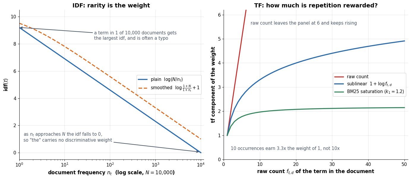
TF-IDF maps each document to a vector whose length equals the vocabulary size, where coordinate $t$ holds a weight that rises with how often term $t$ occurs in that document and falls with how many documents in the corpus contain it. The term-frequency factor is local and per-document, usually damped as $1 + \log f_{t,d}$ so that ten occurrences do not count ten times as much as one. The inverse document frequency factor is a global corpus statistic, $\log(N/n_t)$ , which pushes function words such as “the” toward zero and lifts rare, discriminative terms. Multiplying the two produces the classic “frequent here, rare elsewhere” signal, and L2 normalization turns a plain dot product into cosine similarity. The result is extremely sparse (typically over 99.9% zeros), exactly interpretable per term, and requires no training beyond counting. Its weaknesses are structural rather than fixable by tuning, because every term is its own orthogonal dimension, so “car” and “automobile” share zero similarity, word order and negation are discarded, and any term outside the fitted vocabulary is silently dropped.

(1) Two Factors, Two Scopes: tf is computed from one document, idf from the whole corpus, and the product is what makes a term both present and distinctive.
(2) Sublinear Damping: raw counts overweight repetition, so $1+\log f_{t,d}$ or BM25 saturation caps the reward for saying the same word again.
(3) IDF Is Fitted, Not Computed Per Query: the $n_t$ statistics are frozen at fit time, so corpus drift, duplicated documents, and tiny corpora all distort the weights.
(4) Normalization Removes Length Bias: without L2 (or pivoted) normalization long documents dominate every ranking simply by containing more words.
(5) Sparse Means Cheap And Exact: an inverted index serves lexical matches on CPU in milliseconds, and high idf makes SKUs, error codes, and legal citations very precise.
(6) The Structural Limits: orthogonal vocabulary dimensions mean no synonymy or paraphrase, bag-of-words means no order or negation, and out-of-vocabulary terms contribute nothing at all.

Mathematical Formulation:
$w_{t,d} = \mathrm{tf}(t,d)\cdot \mathrm{idf}(t)$
$\mathrm{tf}(t,d) = 1 + \log f_{t,d}$
$\mathrm{idf}(t) = \log \frac{N}{n_t}$
$\mathrm{idf}_{s}(t) = \log \frac{1+N}{1+n_t} + 1$
$\hat{w}_{d} = w_{d} / \|w_{d}\|_2$
$\mathrm{sim}(q,d) = \hat{w}_{q}^{\top}\hat{w}_{d}$

Where:

$w_{t,d}$ is the unnormalized weight of term $t$ in document $d$ , and $\hat{w}_{d}$ is the final L2-normalized document vector.
$f_{t,d}$ is the raw count of $t$ in $d$ , defined only for $f_{t,d} \geq 1$ ; terms with zero count keep weight zero, which is what makes the vector sparse.
$N$ is the number of documents in the fitted corpus and $n_t$ the document frequency, the number of documents containing $t$ , so $1 \leq n_t \leq N$ .
$\mathrm{idf}_{s}$ is the smoothed variant used by scikit-learn, which adds one to both counts to tolerate unseen terms and adds a constant so a term present everywhere still keeps a small nonzero weight.
$q$ is the query treated as a short pseudo-document, so retrieval scoring is just a cosine between two sparse vectors over shared nonzero coordinates.

Worked IDF Example (natural log, one million documents):
$\mathrm{idf}(\mathrm{the}) = \log(10^6/10^6) = 0$
$\mathrm{idf}(\mathrm{car}) = \log(10^6/10^5) = 2.30$
$\mathrm{idf}(\mathrm{sarcoidosis}) = \log(10^6/50) = 9.90$

The spread of those three numbers is the whole mechanism. A stopword is annihilated without any hand-written stoplist, a common content word keeps a moderate weight, and a domain-specific term is worth roughly four common words in the same document. That also exposes the fragility: a term appearing in exactly one document receives the maximum weight even when it is a typo, an OCR error, or a hash, which is why production pipelines cap the vocabulary with min_df and max_df thresholds instead of trusting idf alone.

Two panels: on the left, inverse document frequency plotted against document frequency on a log x-axis for a corpus of ten thousand documents, comparing the plain log of N over n_t against the smoothed scikit-learn variant, with annotations at the rare-term and stopword ends; on the right, three term-frequency transforms plotted against raw term count, showing the raw linear count leaving the panel, the sublinear one-plus-log curve, and BM25 saturation flattening near two point two

Figure 1: The two factors behave very differently. IDF decays logarithmically in document frequency and reaches zero for a term present in every document, while the tf transform decides how much repetition is rewarded: raw counts grow without bound, $1+\log f_{t,d}$ gives a tenfold count only 3.3 times the weight of a single occurrence, and BM25 saturation is asymptotically bounded by $k_1+1$ .

BM25 is the natural upgrade inside the sparse family, replacing the log-tf term with an explicitly saturating form plus document-length normalization, and it usually beats plain TF-IDF on ranking while keeping the same inverted index. What neither can do is bridge vocabulary mismatch. In a TF-IDF space the coordinates for “car”, “automobile”, and “voiture” are mutually orthogonal, so a query using one word scores exactly zero against a document using another, no matter how many synonyms both share in meaning. Embedding-based representations solve this by construction, mapping text into a dense $\mathbb{R}^{d}$ with $d$ typically between 384 and 1024, where distributional training places related words and paraphrases close together and sub-word tokenization guarantees that nothing is out of vocabulary. The price is real: an encoder needs pretraining plus contrastive fine-tuning, similarity becomes uninterpretable, and dense retrievers can drift badly out of domain, which is exactly where exact lexical matching on an identifier still wins.

Left panel shows a six-term by five-document TF-IDF matrix as a grayscale heatmap with numeric cell values, where the row for the stopword the is all zeros and the rows for car and automobile never share a nonzero column; right panel sketches a dense embedding space as unit arrows from the origin, with car, automobile, and vehicle pointing in nearly the same direction, insurance rotated away, and banana pointing into a different quadrant

Figure 2: Left, a TF-IDF matrix is mostly zeros and each term owns its own axis, so the “car” and “automobile” rows never overlap and their cosine similarity is exactly 0. Right, a dense encoder places the same synonyms at a small angle, which is what recovers paraphrase recall while giving up the per-term readability of the sparse weights.

Property	TF-IDF / BM25 (sparse lexical)	Dense embeddings (bi-encoder)
Dimensionality	Vocabulary size, 50k to 1M, over 99.9% zeros per document	Fixed 384 to 1024 dense floats, fully populated
Fitting cost	One counting pass, no gradients, minutes on CPU	Pretraining plus contrastive fine-tuning on paired data
Synonyms and paraphrase	None: distinct surface forms are orthogonal dimensions	Captured: near-duplicate meanings land at small angles
Rare exact strings	Strong: high idf makes SKUs and error codes highly selective	Weak: rare identifiers are blurred into nearby token directions
Unseen terms	Dropped silently at transform time, contributing nothing	Always representable through sub-word tokenization
Order and negation	Lost, unless n-grams are added at a cost in dimensionality	Partly encoded by the contextual attention layers
Serving	Inverted index, CPU, millisecond lookups, trivial updates	ANN index such as HNSW or IVF, GPU for encoding queries
Dominant failure mode	Vocabulary mismatch gives zero recall on paraphrased queries	Out-of-domain drift returns topically close but wrong documents

August 21, 2026

DL0197 Continuous Incremental Online Learning

What is continuous learning after model deployment, and how do incremental learning and online learning differ in their handling of new data streams and catastrophic forgetting?

Answer

Continuous learning is the practice of keeping a deployed model current as the serving distribution drifts, by updating its parameters from the live stream instead of freezing the artifact that passed offline evaluation. The umbrella covers three regimes that differ in how much data one update sees and how often it ships: periodic batch retraining on the accumulated corpus, incremental learning that resumes from the current weights on a new chunk or task, and online learning that takes one low-learning-rate step per example or micro-batch and never revisits it. Incremental learning still controls the update: it can mix a replay sample of old data into every batch, run a few epochs over the chunk, and gate the result behind a shadow evaluation, so forgetting is a tunable quantity. Online learning gives up that control by construction, because each example is seen once, in arrival order, with no shuffling and no held-out replay, which makes the gradient sequence strongly non-i.i.d. and makes catastrophic forgetting the default rather than the exception. The core tension in both is the stability-plasticity dilemma: enough plasticity to absorb today’s traffic, enough stability to keep yesterday’s competence.

(1) Why Forgetting Happens: gradients computed only on new data are free to move weights that encoded the old distribution, since nothing in the loss references it. Breaking the i.i.d. sampling assumption of SGD is the mechanism, not model capacity.
(2) Incremental Learning Batches The Stream: updates operate on a chunk, task, or day of data, so replay ratios, epoch counts, and evaluation gates are all design knobs.
(3) Online Learning Streams One Pass: a single step per example, bounded memory, and no revisits, which buys seconds-level freshness and pays with instability and high variance.
(4) Three Families Of Mitigation: rehearsal (replay buffers, generative replay), regularization (EWC, distillation from the previous checkpoint), and parameter isolation (adapters, LoRA branches, masks).
(5) Forgetting Is Measurable: report per-task retention and average accuracy from the accuracy matrix, never a single aggregate on fresh traffic, which hides collapse on older slices.
(6) The Dual Failure Is Loss Of Plasticity: a model updated too conservatively for months stops learning at all, so stability alone is not the objective.

Diagram with a live traffic box on the left feeding three horizontal lanes: batch retraining on weeks of shuffled logged data with full offline evaluation and weekly deploys, incremental learning on a new chunk plus a replay sample with a few epochs from current weights and hourly to daily shadow-gated deploys, and online learning taking a single low-learning-rate step per example with learning-rate clipping, canary and rollback guardrails shipping in seconds

Figure 1: The gradient step is identical in all three lanes. What changes is how much data one update sees, how often it ships, and what protects the old distribution: shuffling over the full corpus, an explicit replay sample plus a shadow gate, or nothing but a small learning rate and a rollback button.

In production the choice is usually driven by label latency rather than by an appetite for novelty. Recommendation and ad ranking get feedback in seconds and genuinely benefit from near-online updates, so they run streaming updates on the embedding tables and the last layers while the backbone is refreshed on a slower incremental schedule. Fraud, credit, and medical models often wait days or weeks for a trustworthy label, so a per-example update would be trained on noise; incremental daily or weekly chunks with a replay mix are the safer default. The practical recipe that survives contact with traffic is rarely exotic: keep a stratified replay buffer covering old slices, mix roughly 5 to 20 percent of every batch from it, use a small re-warmed learning rate, and gate every candidate on a fixed regression suite of historical slices before promotion. Parameter isolation is attractive when tasks are known and separable, because a per-task adapter cannot be overwritten, but it grows parameters linearly in the number of tasks and needs task identity at inference unless the routing is learned.

Mathematical Formulation:
$\theta_t = \theta_{t-1} - \eta_t \nabla \ell(\theta_{t-1}; z_t)$
$B_t = \alpha B^{new}_t + (1-\alpha) B^{replay}_t$
$\mathcal{L}(\theta) = \mathcal{L}_{new}(\theta) + \lambda \Omega(\theta)$
$\Omega(\theta) = \tfrac{1}{2}\sum_i F_i (\theta_i - \theta^{*}_i)^2$
$A_K = \frac{1}{K}\sum_{j=1}^{K} a_{K,j}$
$f_j = \max_{k} a_{k,j} - a_{K,j}$

Where:

$\theta_t$ are the parameters after the $t$ -th update, $\eta_t$ the step size, and $z_t = (x_t, y_t)$ the arriving example; the pure online case uses each $z_t$ exactly once.
$B_t$ is the batch actually used at step $t$ , built from fresh data $B^{new}_t$ and a buffer sample $B^{replay}_t$ , with replay ratio $1-\alpha$ typically in the 0.05 to 0.20 range.
$\mathcal{L}_{new}$ is the loss on the incoming chunk and $\Omega$ a stability penalty anchored at the previous checkpoint $\theta^{*}$ , with $\lambda$ trading plasticity for retention.
$F_i$ is the diagonal Fisher information for parameter $i$ under the old task, so weights the old task depended on move less; setting $F_i = 1$ reduces the penalty to plain L2-to-previous.
$a_{k,j}$ is accuracy on task $j$ measured after training through task $k$ , with $j$ and $k$ indexing the $K$ chunks seen so far.
$A_K$ is average accuracy over everything seen and $f_j$ the forgetting on task $j$ , the drop from its best-ever value to its current one.

Figure 2: Sequential updates without rehearsal do not degrade gracefully, they collapse: task 1 loses 69 accuracy points by task 10. A 5 percent replay buffer recovers most of the gap to joint retraining at a fraction of the compute, while a stability penalty alone lands in between because it also suppresses learning on the new chunk.

Property	Batch retraining	Incremental learning	Online learning
Data per update	The full accumulated corpus, shuffled	One chunk, day, or task plus a replay sample	One example or micro-batch, in arrival order
Passes over data	Many epochs, i.i.d. sampling holds	A few epochs inside the chunk, old data only via buffer	Exactly one, no revisits
Freshness	Days to weeks behind traffic	Hours to a day behind	Seconds to minutes behind
Forgetting exposure	None by construction, old data is in every epoch	Bounded and tunable through replay ratio and penalty weight	High, the update sees only the current regime
Main safeguard	Full offline evaluation before promotion	Replay buffer, EWC or distillation, shadow eval on old slices	Small clipped learning rate, canary traffic, instant rollback
Dominant failure	Staleness under drift, and rising retraining cost	Buffer becomes unrepresentative, or the penalty freezes learning	Label noise and feedback loops steer the model within hours
Good fit	Slow drift, regulated or audited models	New domains, languages, or product surfaces arriving over time	Fast implicit feedback such as clicks, prices, or trending content

August 21, 2026

DL0195 Non-Max Suppression

What is Non-Max Suppression (NMS) in object detection, how does it work with confidence scores and IoU thresholds, and what are its limitations and alternatives such as Soft-NMS and DIoU-NMS?

Answer

NMS is the greedy post-processing step that turns a detector’s dense candidate set into a short, non-redundant list of boxes, and it normally runs independently per class. Boxes below a score floor are dropped first, the survivors are sorted by confidence, the highest-scoring box $M$ moves to the output list, and every remaining box whose IoU with $M$ exceeds a threshold $N_t$ is deleted. The loop then repeats on whatever is left: sort → pick the max → suppress → repeat. The algorithm rests on two assumptions, that confidence ranks localization quality and that a high IoU means two boxes describe the same object. Both fail in crowds, where the best box on a partially occluded neighbour can sit above $N_t$ against the winner and is silently erased. Soft-NMS replaces deletion with a monotonic score decay, and DIoU-NMS subtracts a normalized center distance from the IoU so that concentric duplicates are punished harder than offset neighbours.

(1) Greedy Per-Class Loop: NMS is not an optimizer, it is a sorted sweep, so the first mistake it makes is permanent because a deleted box never re-enters the pool.
(2) Two Thresholds, Not One: a score floor (often 0.001 for AP evaluation and 0.25 for a shipped product) plus the IoU threshold $N_t$ in the 0.5 to 0.7 range, with a top- $k$ cap in front to bound the cost.
(3) Confidence Is The Ranking Key: classification score and box quality are only loosely correlated, so NMS can keep a confident but sloppy box and delete a precise one, which is why IoU-aware or centerness-weighted scores improve NMS without touching the algorithm.
(4) Cost: an $O(n \log n)$ sort plus up to $O(n^2)$ pairwise IoU tests, which is why production stacks cap candidates and run a batched CUDA kernel.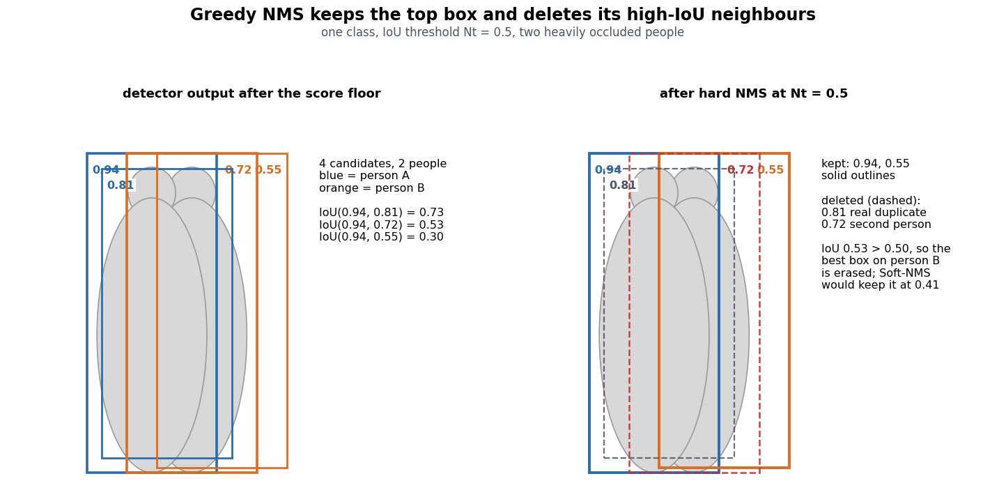
(5) Dominant Failure Mode: a single global $N_t$ must serve sparse and crowded regions of the same image, so lowering it kills recall in crowds and raising it floods sparse regions with duplicates.
(6) Alternatives: Soft-NMS (linear or Gaussian decay), DIoU-NMS (center-distance penalty), Weighted and Cluster-NMS, Matrix NMS, and NMS-free detectors that learn one-to-one assignment instead.

Two side-by-side panels showing a heavily occluded pair of pedestrians. The left panel draws four candidate boxes with confidence scores 0.94 and 0.81 on the first person and 0.72 and 0.55 on the second, with the pairwise IoU values against the top box listed. The right panel shows the result of greedy NMS at IoU threshold 0.5: the 0.94 and 0.55 boxes are kept as solid outlines while the 0.81 duplicate and the 0.72 box on the second person are drawn dashed and grey as suppressed.

Figure 1: Greedy NMS on a heavily occluded pair. The 0.81 box is a genuine duplicate and should go, but the 0.72 box is the detector’s best evidence for the second person, and its IoU of 0.53 with the winner crosses the 0.5 threshold, so hard NMS erases it. What remains for that person is a poorly localized 0.55 box, and Gaussian Soft-NMS would instead keep the 0.72 box at a decayed 0.41.

Mathematical Formulation:
$M = \arg\max_{b_i \in \mathcal{B}} s_i$
$\mathrm{IoU}(M, b_i) = |M \cap b_i| / |M \cup b_i|$
$s_i \leftarrow s_i \cdot \mathbf{1}[\mathrm{IoU}(M, b_i) \leq N_t]$
$s_i \leftarrow s_i \, (1 - \mathrm{IoU}(M, b_i))$
$s_i \leftarrow s_i \exp(-\mathrm{IoU}(M, b_i)^2 / \sigma)$
$\mathrm{DIoU}(M, b_i) = \mathrm{IoU} - \rho^2 / c^2$

Where:

$\mathcal{B}$ is the current candidate set for one class, $b_i$ a box in it with score $s_i$ , and $M$ the current maximum-score box that is moved to the output list $\mathcal{D}$ .
$N_t$ is the IoU threshold; line 3 is hard NMS, which zeroes (deletes) any box overlapping $M$ more than $N_t$ .
Line 4 is linear Soft-NMS, applied only when $\mathrm{IoU}(M, b_i) > N_t$ ; line 5 is Gaussian Soft-NMS, applied to every remaining box with no threshold at all.
$\sigma$ controls the decay width, typically $\sigma = 0.5$ ; a smaller $\sigma$ makes Soft-NMS behave more like hard NMS.
$\rho$ is the Euclidean distance between the two box centers and $c$ the diagonal of the smallest box enclosing both, so $\rho^2 / c^2$ lies in $[0, 1)$ and is scale-invariant.
$i$ indexes the surviving candidates, and the loop terminates when $\mathcal{B}$ is empty or every score falls under the final report floor.

Worked Decay For The Erased Box:
$\mathrm{IoU}(M, b) = 0.53 > N_t = 0.5$
$0.53^2 / 0.5 = 0.5618$
$0.72 \times \exp(-0.5618) = 0.41$

Hard NMS maps that box to 0, Soft-NMS maps it to 0.41, and the practical difference is whether a report threshold of 0.3 still shows the second person. This is also the clearest way to see why Soft-NMS buys roughly 1 to 2 AP on MS COCO with no retraining: average precision rewards a correctly located box even at low confidence, because a decayed detection is ranked below the confident ones and only costs precision after all the good detections are already counted. The same property is a liability in a live product, since nothing is ever deleted and the output list keeps every candidate at some non-zero score, so a final score floor and a top- $k$ cap become mandatory rather than optional.

Line chart with IoU against the kept box on the horizontal axis from 0 to 1 and the score multiplier applied to the overlapping box on the vertical axis from 0 to 1. Hard NMS is a step function that holds at 1 until IoU 0.5 and then drops to 0. Linear Soft-NMS holds at 1 until 0.5 and then falls linearly to 0 at IoU 1. Gaussian Soft-NMS with sigma 0.5 decays smoothly from 1 and reaches about 0.14 at IoU 1, with an annotation marking that IoU 0.53 keeps 57 percent of the score.

Figure 2: Every NMS variant is just a different score multiplier as a function of IoU. Hard NMS is a discontinuous step at $N_t$ , which is what makes a 0.499 and a 0.501 overlap have completely different fates. Soft-NMS swaps the step for a monotonic decay, so the cliff at the threshold disappears and the ranking, rather than a hard rule, decides what appears in the final list.

DIoU-NMS attacks a different weakness: IoU alone cannot tell a concentric duplicate from a genuinely different object. Two boxes that share a center almost certainly describe the same thing, while two boxes with the same IoU but far-apart centers are much more likely to be neighbouring instances, so the criterion becomes IoU minus the squared center distance normalized by the enclosing diagonal. The catch is that same normalization. For two tall, near-identical pedestrian boxes offset by a fraction of their width, $\rho^2 / c^2$ is on the order of 0.01, so DIoU-NMS behaves almost exactly like hard NMS on the case in Figure 1. It helps most where scale or center offset differs substantially, which is why it is usually reported together with the DIoU regression loss rather than as a standalone fix for crowds.

Two panels each showing a large kept box M with a candidate box. In the left panel the candidate is a smaller box concentric with M, both centers coincide, IoU is 0.25, the center distance is zero and DIoU stays 0.25 so the box is suppressed at a 0.20 threshold. In the right panel the candidate is the same size as M but shifted horizontally, IoU is again 0.25, the center distance is 3.6 with the dashed enclosing box diagonal marked, the penalty is 0.10 and DIoU falls to 0.15 so the box is kept.

Figure 3: Both candidates have identical IoU 0.25 with the kept box, so hard NMS treats them identically. DIoU-NMS separates them: the concentric box keeps DIoU 0.25 and is deleted, while the offset box pays a 0.10 penalty and survives at 0.15 under a 0.20 threshold. Because the penalty is divided by the enclosing-box diagonal, it only bites when the center offset is large relative to the pair’s extent.

Property	Hard NMS	Soft-NMS	DIoU-NMS
Rule on an overlapping box	Delete if IoU exceeds Nt	Multiply the score by a linear or Gaussian decay, never delete	Delete if IoU minus the normalized center distance exceeds the threshold
Hyperparameters	Nt only, usually 0.5 to 0.7	Decay form, sigma near 0.5, plus a mandatory final score floor	Threshold plus the implicit distance normalization (sometimes an exponent beta)
Output size	Bounded and small	Every candidate survives with some score, so top-k is required	Bounded, slightly larger than hard NMS
Crowded scenes	Worst case, deletes true neighbours outright	Best AP gain, roughly 1 to 2 AP on MS COCO with no retraining	Helps when centers differ; near no effect for side-by-side boxes of equal size
Cost	Sort plus pairwise IoU, fast batched CUDA kernel	Same order but no early deletion, so more IoU work and a longer output list	Hard NMS plus one center-distance term per pair
Typical use	Default in Faster R-CNN and YOLO inference paths	Benchmark AP, crowd and dense-object settings, offline pipelines	Shipped with the DIoU/CIoU loss family, for example YOLOv4

The deeper limitation is structural rather than parametric: NMS is a non-differentiable, hand-tuned rule bolted onto a learned model, so the network is never trained to produce exactly one box per object. That is what NMS-free detectors remove. DETR-style models use Hungarian one-to-one matching during training, so duplicate suppression becomes a learned property of the decoder, and YOLOv10 keeps a one-to-many head for training signal while using a one-to-one head at inference, eliminating the NMS stage and its latency variance entirely.

August 21, 2026

DL0191 GCN, GraphSAGE, and GAT

How do Graph Convolutional Networks (GCN), GraphSAGE, and Graph Attention Networks (GAT) differ in their neighborhood aggregation strategies, and what are the trade-offs in transductive versus inductive settings?

Answer

All three layers do the same thing at a high level: build a new vector for node $i$ as a weighted combination of its neighbors’ vectors, then apply a linear map and a nonlinearity. The real difference is where the mixing coefficient comes from and how the neighborhood is enumerated. GCN fixes the coefficient from the graph alone as symmetric degree normalization $1/\sqrt{\tilde{d}_i \tilde{d}_j}$ , applied to the full neighborhood in one sparse matrix product over the entire graph. GraphSAGE replaces the full neighborhood with a fixed-size random sample and a permutation-invariant aggregator (mean, max-pool, or LSTM), and keeps the node’s own vector in a separate concatenated slot instead of averaging it away. GAT makes the coefficient content-dependent: a small shared scoring vector reads both endpoint features, a softmax over each node’s neighborhood turns those scores into weights $\alpha_{ij}$ , and several attention heads are run in parallel. Transductive versus inductive is then mostly a property of the training procedure and of what the coefficients depend on, not of the layer equation itself.

(1) GCN Weights Are Structural And Frozen: $c_{ij}$ depends only on the two degrees, so a high-degree hub is deliberately down-weighted and no coefficient is ever learned. This is a strong, cheap prior when features are weak and the graph is homophilous.
(2) GraphSAGE Weights Are Uniform Over A Sample: the mean aggregator gives every sampled neighbor $1/|S(i)|$ , and the sample size is the knob that bounds compute rather than the node’s true degree.
(3) Self Vector Handling Differs: GCN and GAT fold the node into the same sum through a self-loop, while GraphSAGE concatenates it and gives it its own block of the weight matrix, which preserves the node’s own signal at depth.
(4) GAT Weights Are Learned From Features: $\alpha_{ij}$ can vary across edges of identical degree, which is what lets the layer ignore a noisy neighbor. The price is $K|E|$ stored coefficients and gradients flowing through the attention scores.
(5) Transductive Is A Training Choice, Not A Law: the published GCN is trained full-batch on a single normalized adjacency, so a new node changes degrees and the normalization; GraphSAGE was designed minibatch-first so the same weights run on an unseen node by sampling its fan-out.
(6) Depth Costs Differently: full-neighborhood expansion grows as roughly $\bar{d}^{\,L}$ per target node, while sampling caps it at $\prod_l S_l$ at the cost of estimator variance.

Three side-by-side panels showing the same target node with four neighbors A, B, C, D. In the GCN panel the incoming arrow thickness follows fixed degree-based coefficients 0.32, 0.26, 0.18 and 0.15 with a self-loop coefficient 0.20. In the GraphSAGE panel only A and C are sampled with equal weight 0.50, B and D are drawn as dashed gray unsampled nodes, and the target keeps its own vector through concatenation. In the GAT panel the coefficients are learned attention values 0.09, 0.46, 0.11, 0.19 with self attention 0.15, so arrow thickness no longer tracks degree.

Figure 1: One neighborhood, three weighting rules. GCN reads its coefficients off the degrees, so the sparsest neighbor A gets the largest share and the hub D the smallest. GraphSAGE throws away two neighbors and splits the mass uniformly over what survives, keeping the self vector in a separate concatenated slot. GAT lets features decide, so neighbor B dominates with $\alpha = 0.46$ despite having a middling degree.

Mathematical Formulation:
$h_i' = \sigma\big(\textstyle\sum_{j \in \tilde{N}(i)} c_{ij} W h_j\big)$
$c_{ij} = 1 / \sqrt{\tilde{d}_i \tilde{d}_j}$
$a_i = \mathrm{AGG}(\{h_j : j \in S(i)\})$
$h_i' = \sigma(W \, [\, h_i \,\|\, a_i \,])$
$e_{ij} = \mathrm{LeakyReLU}(a^{\top}[W h_i \,\|\, W h_j])$
$\alpha_{ij} = \mathrm{softmax}_j(e_{ij})$
$h_i' = \sigma\big(\textstyle\sum_{j \in \tilde{N}(i)} \alpha_{ij} W h_j\big)$

Where:

$h_i \in \mathbb{R}^{d}$ is the incoming representation of node $i$ and $h_i'$ the layer output; $\sigma$ is the elementwise nonlinearity and $W$ the shared linear map.
$\tilde{N}(i)$ is the neighborhood including the self-loop, and $\tilde{d}_i$ is the corresponding degree, so $c_{ij}$ is the fixed GCN coefficient that never changes during training.
$S(i) \subseteq N(i)$ is the sampled fan-out of fixed size $S_l$ at layer $l$ , and $\mathrm{AGG}$ is a permutation-invariant reducer (mean, elementwise max over an MLP, or LSTM over a shuffled order).
$\|$ is concatenation, so the GraphSAGE weight matrix has shape $d' \times 2d$ and the node’s own features get an independent parameter block.
$a \in \mathbb{R}^{2d'}$ is the shared attention vector and $e_{ij}$ the raw score; the softmax is taken over $j \in \tilde{N}(i)$ so that $\sum_j \alpha_{ij} = 1$ per node.
GAT runs $K$ heads whose outputs are concatenated in hidden layers and averaged in the output layer, multiplying both parameter count and stored coefficients by $K$ .

The cost picture follows directly. A full-batch GCN layer is $O(|E| d + |V| d^2)$ and needs the whole feature matrix plus every layer’s activations resident, which is why it stops fitting long before the graph itself does. GAT adds $O(K |E|)$ scores and their gradients on top of the same sparse pattern, so its memory is edge-bound rather than node-bound. GraphSAGE instead bounds a minibatch: with batch size $B$ and fan-outs $(S_1, \ldots, S_L)$ , the computation graph holds a number of node instances that is completely independent of $|V|$ . That is the property that makes web-scale graph learning practical, and it is the mechanism behind Pinterest’s PinSage, which trains on a graph of billions of nodes by expanding only short sampled neighborhoods per target.

Minibatch Fan-Out Budget:
$N_{mb} = B \prod_{l=1}^{L} S_l$
$25 \times 10 = 250$
$N_{mb} = 512 \times 250 = 128000$

Log-scale line chart of node instances in the computation graph for a single target node versus GNN depth from 1 to 4 layers. Full-neighborhood expansion at average degree 100 rises from 100 to about 101 million, full-neighborhood expansion at average degree 20 rises from 20 to about 168 thousand, and sampled fan-out 25 then 10 per layer rises only from 25 to about 28 thousand. A dashed horizontal line marks a graph of 2.4 million nodes, which the average-degree-100 curve crosses between three and four layers.

Figure 2: Depth is what makes full-neighborhood aggregation intractable. On a graph with average degree 100, a 3-hop receptive field already touches about a million node instances per target and a 4-hop field exceeds the graph size, meaning most of the graph is re-visited for a single prediction. A fixed fan-out of 25 then 10 keeps the same depth at roughly 2,800 instances, trading exactness for a cost that no longer depends on $|V|$ .

Property	GCN	GraphSAGE	GAT
Neighbor weight	Fixed 1 / sqrt(d_i d_j)	Uniform 1 / \|S(i)\|, or max-pool / LSTM reducer	Learned alpha_ij per head, softmax over the neighborhood
Weight depends on	Graph structure only	Sample size only	Endpoint features, so it changes as the model trains
Self representation	Self-loop term inside the same sum	Concatenated, own block of the weight matrix	Self-loop with its own attention coefficient
Published training regime	Full-batch over one normalized adjacency	Minibatch with fixed per-layer fan-out sampling	Full-batch on citation graphs, sampled variants for large graphs
Unseen node at inference	Degrees and normalization must be recomputed; the transductive recipe assumes the test nodes were present during training	Designed for it: sample the fan-out and run one forward pass	Works if the new node has features, since attention is edge-local
Per-layer cost	O(\|E\| d + \|V\| d^2), memory scales with the whole graph	O(B x prod S_l x d) per batch, independent of \|V\|	K x O(\|E\| d), plus K\|E\| stored coefficients and their gradients
Dominant failure mode	Over-smoothing beyond two or three layers; hubs are dampened by construction	Sampling variance and unstable embeddings; fan-out explodes at three or more layers	Edge-bound memory; static attention ranking, which GATv2 fixes

August 20, 2026

DL0190 GNN Message Passing Paradigm

What is the Message Passing Paradigm in Graph Neural Networks, and how does it unify node, edge, and graph-level predictions through neighborhood aggregation and update functions?

Answer

Message passing is the observation that almost every graph neural network layer can be written as three functions applied in the same order: a message function that runs once per edge, a permutation-invariant aggregation over each node’s neighborhood, and an update function that mixes the aggregate with the node’s previous state. Stacking $K$ such layers gives every node a representation that summarizes its $K$ -hop neighborhood, so depth and receptive field are the same knob. GCN, GraphSAGE, GAT, and GIN differ only in how they instantiate the message and the aggregator, which is why one implementation of the scatter-gather loop covers all of them. The unification across prediction granularities is equally mechanical, because the encoder is identical in all three cases and only the readout changes: a node label reads $h_v$ directly, an edge or link score reads the pair $(h_u, h_v)$ , and a graph label reads a pooled summary of all node states. Training therefore differs in the loss and label granularity, not in the architecture.

(1) Message Function: $\phi$ runs once per directed edge and may use the source state, the target state, and the edge features, which is how bond types or relation types enter the computation.
(2) Permutation-Invariant Aggregation: the neighborhood is an unordered multiset, so $\bigoplus$ must be sum, mean, max, or attention-weighted sum; anything order-dependent makes the layer ill-defined.
(3) Update Function: $\psi$ combines the old state with the aggregate, usually a linear map plus nonlinearity, and in deep stacks a residual connection to keep the node’s own signal alive.
(4) Depth Equals Receptive Field: after $K$ rounds a node has seen exactly its $K$ -hop subgraph, so long-range tasks need either depth or a shortcut mechanism.
(5) One Encoder, Three Heads: node, edge, and graph predictions are three readouts over the same embedding matrix, which lets you pretrain on one granularity and fine-tune on another.
(6) Cost Scales With Edges: a layer is $O(|E|d + |V|d^2)$ , sparse in the graph and independent of the diameter, which is why message passing scales where dense pairwise attention does not.

Diagram of one message passing layer: a small graph on the left with a target node v receiving solid message arrows from three neighbors and dashed edges to two-hop nodes, feeding a three-box pipeline on the right labeled message function phi per edge, permutation-invariant aggregation with sum mean or max, and update function psi producing the new node state

Figure 1: One layer, three functions. Every incident edge produces a message, the messages collapse into a single vector through a permutation-invariant operator, and the update mixes that vector with the node’s previous state. The dashed two-hop nodes contribute nothing at this layer; they only reach $v$ after a second round, which is what makes depth and receptive field the same quantity.

The reason this paradigm generalizes so well is that it commits to locality and permutation equivariance and nothing else. There is no assumption of a fixed node ordering, a fixed degree, or a fixed graph size, so the same trained weights apply to a 12-atom molecule and a 40-atom molecule. The interesting design freedom sits in the aggregator. Mean pooling normalizes away degree, which helps on citation graphs where degree is a popularity artifact and hurts on tasks where the count itself is the signal. Sum pooling keeps the count and is what makes GIN as discriminative as the 1-Weisfeiler-Lehman test, the theoretical ceiling for standard message passing. Max pooling behaves like a feature detector and is robust to noisy neighbors but blind to multiplicity.

Mathematical Formulation:
$m_{uv}^{(k)} = \phi^{(k)}(h_v^{(k-1)}, h_u^{(k-1)}, e_{uv})$
$a_v^{(k)} = \bigoplus_{u \in \mathcal{N}(v)} m_{uv}^{(k)}$
$h_v^{(k)} = \psi^{(k)}(h_v^{(k-1)}, a_v^{(k)})$
$h_G = R(\{ h_v^{(K)} : v \in V \})$

Where:

$h_v^{(k)} \in \mathbb{R}^{d}$ is the state of node $v$ after $k$ rounds, with $h_v^{(0)}$ the input node features.
$m_{uv}^{(k)}$ is the message sent from neighbor $u$ to $v$ , and $a_v^{(k)}$ is the aggregated neighborhood vector.
$\phi^{(k)}$ and $\psi^{(k)}$ are the learned message and update functions, typically small MLPs or a single linear layer with a nonlinearity.
$\bigoplus$ is a permutation-invariant operator over a multiset, most often sum, mean, or max.
$\mathcal{N}(v)$ is the neighbor set of $v$ and $e_{uv}$ the optional edge feature vector.
$k \in \{1, \ldots, K\}$ indexes rounds, so $K$ is both the layer count and the hop radius of the receptive field.
$R$ is the graph readout, itself permutation invariant, producing the whole-graph vector $h_G$ .

Diagram showing an input graph feeding a stack of K message passing layers that produces a node embedding matrix, which then branches into three heads: a node head applied per node, an edge head applied to the concatenation of two endpoint embeddings, and a graph head applied after a permutation-invariant readout pooling

Figure 2: The encoder is shared and only the readout changes. Node classification consumes $h_v$ , link prediction consumes a symmetric function of the endpoint pair, and graph regression consumes a pooled summary. This is why a single library implements all three task families with one message passing loop and three thin heads.

The Three Readouts:
$\hat y_v = f_n(h_v^{(K)})$
$\hat y_{uv} = f_e([h_u^{(K)} ; h_v^{(K)}])$
$\hat y_G = f_g(h_G)$

For link prediction the pair function should be symmetric on undirected graphs, so practitioners use the Hadamard product $h_u \odot h_v$ or a dot product rather than a raw concatenation, which is order-dependent unless both orders are trained. A concrete instantiation makes the abstraction less slippery. GCN takes the message to be a degree-normalized copy of the neighbor state and folds the update into one linear map:

GCN As A Message Passing Layer:
$c_{uv} = 1 / \sqrt{d_u d_v}$
$h_v^{(k)} = \sigma \Big( W^{(k)} \sum_{u \in \tilde{\mathcal{N}}(v)} c_{uv} h_u^{(k-1)} \Big)$
$\text{cost} = O(K|E|d + K|V|d^2)$

Here $d_u$ is the degree of $u$ and $\tilde{\mathcal{N}}(v)$ includes $v$ itself through the self-loop, so GCN is a fixed-coefficient weighted mean with no learned message. GAT replaces $c_{uv}$ with a learned attention weight, GraphSAGE concatenates the self state instead of summing it in, and GIN uses a sum with an MLP update. Only the choice of $\phi$ , $\bigoplus$ , and $\psi$ changes.

Property	Sum	Mean	Max
Keeps degree information	Yes, the magnitude grows with degree	No, degree is normalized away	No, only the strongest signal survives
Distinguishes multisets	Injective with an MLP update, so 1-WL expressive (GIN)	Confuses {a, a} with {a}	Confuses {a, b} with {a, b, b}
Scale stability	Poor on heavy-tailed degrees, needs normalization	Good, activations stay bounded	Good, but gradients reach one neighbor only
Typical use	Molecular property prediction where atom counts matter	Citation and social graphs with hub nodes	Point clouds and noisy neighborhoods

Two structural limits follow directly from the paradigm rather than from any particular implementation. Over-smoothing means that repeated neighborhood averaging drives node states toward a low-dimensional, degree-dependent subspace, so accuracy on node tasks often peaks at 2 to 4 layers. Over-squashing means that a node’s $K$ -hop neighborhood can grow exponentially while its state stays a fixed $d$ -vector, so information from distant nodes is compressed through bottleneck edges and effectively lost. Both are reasons that deeper is not automatically better, and both motivate residual connections, jumping-knowledge readouts, graph rewiring, and virtual global nodes.

August 20, 2026

DL0182 Semantic, Instance, and Panoptic Segmentation

What are the differences between Semantic, Instance, and Panoptic Segmentation, and when is each task formulation used in practice, for example inside an autonomous-driving perception stack?

Answer

The three tasks differ in what a label is allowed to be. Semantic segmentation assigns every pixel exactly one class out of $K$ and has no notion of object identity, so two touching cars collapse into a single connected “car” region. Instance segmentation does the opposite: it detects and masks each countable object separately with a confidence score, but it only covers thing classes, ignores amorphous stuff such as road, sky, and vegetation, and its masks may overlap each other or leave pixels uncovered. Panoptic segmentation is the union of the two: every pixel receives one pair $(c_p, z_p)$ of class plus instance id, stuff classes get a single segment with no id, things get one segment per object, and the output is a strict partition of the image with no overlaps and no unlabeled pixels except an explicit void region. Which formulation you pick follows the consumer of the output, not fashion. A planner that needs to count and track individual vehicles needs ids, whereas a free-space or sky-replacement module only needs a region mask.

(1) Label Space: semantic returns a class per pixel, instance returns a set of scored binary masks with classes, and panoptic returns a class plus an id per pixel.
(2) Things Versus Stuff: instance segmentation is defined only on countable things; semantic segmentation handles both but cannot separate two instances; panoptic handles both and separates instances.
(3) Overlap Constraint: instance masks are independent and can overlap, while panoptic forces a non-overlapping partition, which means any fusion of two heads must resolve conflicts explicitly.
(4) Metrics Differ In Kind: semantic uses mIoU, instance uses mask AP averaged over IoU thresholds and scores, and panoptic uses PQ at a single fixed matching threshold with no score sweep.
(5) Annotation Cost: stuff-only masks are cheap polygon paint, per-instance boundaries between adjacent same-class objects are the most expensive labels in the dataset.
(6) Practical Selection: use semantic for region questions, instance for counting and tracking, and panoptic when a downstream module needs one consistent scene interpretation per pixel.

Three panels showing the same toy scene of sky, road, two touching cars, and a person labeled three ways: semantic where both cars form one car region, instance where only the two cars and the person get scored masks that slightly overlap while sky and road are ignored, and panoptic where every pixel receives one class plus instance id with the two cars separated by a hard boundary

Figure 1: One scene, three label spaces. The interesting pixels are the ones on the boundary between the two touching cars: semantic segmentation is structurally unable to place that boundary, instance segmentation places it but may let the two masks overlap and says nothing about road or sky, and panoptic segmentation is required to place it and to label every remaining pixel exactly once.

In practice the formulation is chosen by the consumer. Free-space and drivable-area estimation, land-cover mapping from satellite imagery, portrait or sky matting, and organ or tumor delineation are region questions, so semantic segmentation is sufficient and its cheaper labels are a real advantage. Counting, tracking, and grasping are identity questions: counting cells in a microscopy image, tracking each pedestrian across frames, or picking one item out of a bin all require per-object masks, so instance segmentation (or its video extension) is the right task. Panoptic segmentation earns its extra cost when a single downstream consumer must be handed one coherent interpretation of every pixel, which is why it is the natural output format for driving perception and robot scene understanding, where the same map must answer both “is this pixel drivable” and “which vehicle is this”. A useful diagnostic question is whether two adjacent objects of the same class must ever be told apart. If the answer is no, panoptic annotation is money spent on a distinction nobody reads.

Mathematical Formulation:
$f_{\mathrm{sem}}(p) = c_p$
$f_{\mathrm{ins}} = \{(m_j, c_j, s_j)\}_{j=1}^{M}$
$f_{\mathrm{pan}}(p) = (c_p, z_p)$
$\mathrm{mIoU} = \frac{1}{K}\sum_{k=1}^{K}\frac{TP_k}{TP_k + FP_k + FN_k}$
$\mathrm{PQ} = \mathrm{SQ} \times \mathrm{RQ}$
$\mathrm{SQ} = \frac{1}{|TP|}\sum_{(g,q) \in TP}\mathrm{IoU}(g,q)$
$\mathrm{RQ} = \frac{|TP|}{|TP| + \frac{1}{2}|FP| + \frac{1}{2}|FN|}$

Where:

$p$ is a pixel, $c_p$ its class, and $z_p$ its instance id, which is undefined (shared) for stuff classes and unique per object for thing classes.
$K$ is the number of classes, split into disjoint thing and stuff subsets by the dataset definition rather than by the model.
$m_j$ is the $j$ -th predicted binary mask, $c_j$ its class, and $s_j$ its confidence; the $M$ masks are independent, so they may overlap and their union need not cover the image.
$TP$ , $FP$ , and $FN$ in PQ count segments, not pixels, with a ground-truth segment $g$ and a prediction $q$ matched when $\mathrm{IoU}(g,q) > 0.5$ ; that threshold makes the matching provably unique because panoptic segments cannot overlap.
$\mathrm{SQ}$ is segmentation quality, the mean IoU of matched pairs, and $\mathrm{RQ}$ is recognition quality, the F1 score over segments; PQ is reported per class and then averaged, and often split into $\mathrm{PQ}^{\mathrm{th}}$ and $\mathrm{PQ}^{\mathrm{st}}$ .
$TP_k$ in mIoU counts pixels of class $k$ , which is why mIoU is blind to how many objects a class region contains.

Worked Example (One Image):
$\mathrm{SQ} = 3.10 / 4 = 0.775$
$\mathrm{RQ} = 4 / (4 + 1 + 1) = 0.667$
$\mathrm{PQ} = 0.775 \times 0.667 = 0.517$

Four matched segments whose IoUs sum to 3.10 give an SQ of 0.775, and two false positives plus two false negatives each contribute a half count to the RQ denominator, so RQ is 0.667 and PQ lands at 0.517. The decomposition is the practically useful part: a high SQ with a low RQ means the masks are accurate but segments are being missed or hallucinated, which points at the classification and duplicate-removal path, while a high RQ with a low SQ means the right objects are found with sloppy boundaries, which points at output resolution and boundary supervision.

Diagram of panoptic quality computation with a left column of six ground-truth segments and a right column of six predicted segments, arrows joining four matched pairs labeled with IoU values 0.92, 0.81, 0.74 and 0.63, a red dashed pair at IoU 0.38 that fails the threshold and counts as both a false positive and a false negative, one unmatched ground-truth sky segment, one spurious truck prediction, and a side panel computing SQ 0.775, RQ 0.667 and PQ 0.517

Figure 2: PQ is a segment-level bipartite matching followed by a product of two interpretable factors. The pair at IoU 0.38 is the detail that separates candidates who have read the metric from those who have not: it is not a weak match, it is no match at all, and it is charged once as a false positive and once as a false negative.

Property	Semantic	Instance	Panoptic
Output per pixel	One class id	Zero, one, or several scored masks	Exactly one (class, instance id) pair
Stuff classes	Covered	Not part of the task	Covered as one segment per class
Separates same-class objects	No	Yes	Yes, and mandatory
Overlapping masks	Impossible by construction	Allowed and common	Forbidden, conflicts must be resolved
Standard metric	mIoU over pixels	Mask AP swept over IoU and score	PQ = SQ x RQ at IoU above 0.5
Classic architecture	FCN, DeepLab, per-pixel softmax	Mask R-CNN, box then mask head	Panoptic FPN, or mask-classification with queries
Typical use	Free space, land cover, matting, organ delineation	Counting, tracking, robotic grasping	Driving and robot scene understanding, one map for all consumers

August 20, 2026

DL0178 SAM: Promptable Segmentation

How does SAM (Segment Anything Model) use promptable Vision Transformer encoders for zero-shot object segmentation, and what makes its prompt interface generalizable to unseen object categories?

Answer

SAM splits segmentation into one expensive image step and a very cheap prompt step. A ViT-H image encoder (MAE-pretrained, about 632M parameters) takes a 1024×1024 image, converts it into $64 \times 64$ patch tokens, and emits a single image embedding of shape $64 \times 64 \times 256$ that is computed once and cached. A tiny prompt encoder maps whatever the user supplies (clicks, a box, a coarse mask, text) into 256-dimensional tokens, and a two-block two-way cross-attention mask decoder reads the cached embedding together with those tokens to produce three mask logits plus three predicted IoU scores in roughly 50 ms. Generalization to unseen categories comes from the task definition rather than from any category machinery: the objective is “return a valid mask for this prompt”, there is no classification head and no fixed label set, so the model only ever learns a geometry-to-region mapping, supervised by 1.1B masks over 11M images (SA-1B) that a model-in-the-loop data engine collected without class labels. The one thing a category-free interface cannot resolve is ambiguity, and SAM handles it by predicting three nested candidates and back-propagating only the lowest-loss one.

(1) Asymmetric Compute: the ViT encoder runs once per image (about 0.15 s on a GPU) while the decoder runs once per prompt (about 50 ms, light enough for a browser), which is what makes interactive clicking feasible.
(2) Prompts Become Tokens: points and boxes are Fourier positional encodings of their coordinates plus a learned type embedding; a coarse mask prompt is instead embedded by a small convolutional stack and added elementwise to the image embedding.
(3) Two-Way Attention Decoder: prompt tokens attend to image features and image features attend back to the tokens, so a handful of tokens can reshape a dense 4096-token feature map at negligible cost.
(4) Dynamic Mask Head: each mask token is turned by an MLP into the weights of a linear classifier that is dotted with the 4x-upscaled embedding, so the mask is produced by a per-prompt hypernetwork rather than by fixed per-class filters.
(5) Ambiguity-Aware Output: three masks (subpart, part, whole) with a min-over-masks loss and an IoU-prediction token for ranking, which prevents the averaging that destroys single-output models on ambiguous clicks.
(6) Composable Interface: because the prompt is only geometry, any upstream module can drive SAM (a detector’s box, a CLIP text embedding, or a regular grid of points for fully automatic mask generation) with no retraining.

Architecture diagram showing an input image passing through a ViT-H encoder into a cached 64 by 64 by 256 image embedding on the top row, prompts passing through a small prompt encoder into prompt tokens plus three mask tokens and one IoU token on the bottom row, a dashed path where a dense mask prompt is convolved and added to the image embedding, both paths feeding a lightweight two-block two-way cross-attention mask decoder, which outputs three mask logits and three predicted IoU scores

Figure 1: The whole design is an amortization argument. Everything expensive is a function of the image alone and is cached; everything that depends on the prompt is a few million parameters of decoder. Note the absence of any classification branch: the output is a region and a quality score, never a category.

The reason this interface transfers to categories that never appeared in training is that the prompt carries no semantics at all. A click is a coordinate, a box is two coordinates, and the encoder was pretrained to represent generic visual structure, so segmenting a species of coral or an industrial part reuses exactly the same computation as segmenting a cat. What must be learned instead is the notion of “object-ness at the scale the prompt implies”, and SA-1B provides that at massive scale precisely because its data engine was label-free: annotators clicked regions, then a partially trained SAM proposed masks that annotators only corrected, then the final stage generated masks automatically from a $32 \times 32$ point grid with NMS and stability filtering. Ambiguity is the residual difficulty. A single click on a shirt pocket is consistent with the pocket, the shirt, and the person, so a single-output model trained with an averaged loss learns a blurred compromise. SAM emits three masks and only the one with the lowest loss receives gradient, which forces the three slots to specialize by scale.

Three side-by-side stylized figures of a person wearing a shirt with a pocket, each marked by the same star-shaped point prompt on the pocket; the first panel highlights only the pocket as the subpart mask, the second highlights the shirt as the part mask, the third highlights the entire person as the whole mask, each labeled with a different predicted IoU score

Figure 2: One prompt, three valid answers. The min-over-masks loss back-propagates only through whichever slot best matches the ground-truth region, so slot 1 drifts toward subparts, slot 2 toward parts, and slot 3 toward whole objects. The IoU-prediction token then supplies the ranking the interface needs when no human is in the loop.

Mathematical Formulation:
$F = E_{\mathrm{img}}(I) + \mathrm{conv}(m)$
$p_k = \mathrm{PE}(x_k, y_k) + t_{\mathrm{type}(k)}$
$P = (p_1, \ldots, p_{N_p}, o_1, o_2, o_3, o_{\mathrm{iou}})$
$(Z, H) = \mathrm{Dec}(F, P)$
$M_j = \langle \mathrm{MLP}_j(H), \mathrm{Up}_4(Z) \rangle$
$\mathcal{L}_j = 20\,\ell_{\mathrm{focal}}(M_j) + \ell_{\mathrm{dice}}(M_j)$
$\mathcal{L} = \min_{j \in \{1,2,3\}} \mathcal{L}_j$

Where:

$F \in \mathbb{R}^{64 \times 64 \times 256}$ is the cached image embedding, $E_{\mathrm{img}}$ the ViT-H encoder applied to the 1024×1024 image $I$ , and $m$ an optional coarse mask prompt whose convolutional embedding is added elementwise.
$p_k$ is the token for sparse prompt $k$ , built from a random Fourier positional encoding $\mathrm{PE}$ of its coordinates plus a learned embedding $t_{\mathrm{type}}$ for foreground point, background point, box corner, or text.
$P$ is the decoder’s token sequence: $N_p$ prompt tokens plus three learned mask tokens $o_j$ and one IoU token $o_{\mathrm{iou}}$ .
$Z$ is the updated image feature map and $H$ the updated tokens after two blocks of two-way cross-attention; $\mathrm{Up}_4$ is a pair of transposed convolutions giving a $256 \times 256$ map.
$M_j$ is mask $j$ ‘s logit map, formed by dotting the dynamically predicted weights $\mathrm{MLP}_j(H)$ with every spatial location of $\mathrm{Up}_4(Z)$ , then bilinearly resized to 1024×1024.
$\ell_{\mathrm{focal}}$ and $\ell_{\mathrm{dice}}$ are combined in a 20:1 ratio, and only the argmin slot receives gradient; the IoU head is trained separately with an MSE loss against the realized IoU.

Latency Accounting For $K$ Prompts On One Image:
$C_{\mathrm{enc}} = O(N^2 d), \quad N = 4096$
$C_{\mathrm{dec}} = O(N_t N d)$
$T(K) = t_{\mathrm{enc}} + K \, t_{\mathrm{dec}}$
$T(32) = 150\ \mathrm{ms} + 32 \times 50\ \mathrm{ms}$
$T(32) = 1750\ \mathrm{ms}$

The quadratic term belongs entirely to the encoder over $N = 4096$ tokens, while the decoder is linear in the $N_t \approx 8$ tokens it carries, which is why 32 clicks cost 1.75 s with caching but 6.4 s if the ViT is re-run each time. Automatic mask generation exploits the same asymmetry: a $32 \times 32$ grid of 1,024 point prompts, run in batches against one cached embedding, yields a full mask inventory for the image without ever re-encoding it.

Line chart of total latency in milliseconds versus number of prompts on a single image, comparing a caching design that pays 150 milliseconds once plus 50 milliseconds per prompt against a design that re-runs the encoder for every prompt at 200 milliseconds each, with an annotation marking 1.75 seconds versus 6.4 seconds at 32 prompts

Figure 3: Why the encoder/decoder split is the architecture, not an optimization. Caching turns the marginal cost of a prompt from 200 ms into 50 ms, and the gap widens with every additional click, which is exactly the regime an interactive annotation tool or a 1,024-point automatic sweep lives in.

Property	Point clicks	Box	Coarse mask	Text
Encoding path	Sparse: Fourier positional encoding plus fg/bg type embedding	Sparse: two corner tokens with corner-specific embeddings	Dense: conv stack added elementwise to the image embedding	Sparse: a CLIP text embedding used as one token
What it pins down	Location only, so scale stays ambiguous	Location and extent, which resolves most ambiguity	Full spatial support, used for iterative refinement	Semantics with no localization
Typical source	Human clicks, or a 32×32 grid for automatic generation	An upstream detector such as Grounding DINO	SAM’s own previous output in a refinement loop	A user query in the exploratory prototype
Main failure mode	Wrong scale slot chosen when no human ranks the three masks	Loose or overlapping boxes leak into neighboring instances	Errors in the input mask are reinforced across iterations	Weakest of the four; not a released production interface

August 19, 2026

DL0177 Discrete vs Continuous Visual Tokens

What is the difference between discrete visual tokenization (e.g., VQ-VAE, VQ-GAN) and continuous vision embeddings (e.g., ViT patch outputs), and when is each preferred for generation versus understanding tasks?

Answer

Both paths begin identically, with a convolutional or ViT encoder turning the image into a grid of $d$ -dimensional vectors. The only structural difference is whether a quantizer follows. A discrete tokenizer (VQ-VAE, VQ-GAN) snaps each vector to its nearest entry in a learned codebook of $K$ vectors and keeps only the integer index, so an image becomes a string of ids over a finite vocabulary that a jointly trained decoder can invert back to pixels. A continuous representation (ViT patch outputs, CLIP or SigLIP features, KL-VAE latents) keeps the float vector, which preserves far more information but has no finite support, so no softmax and no cross-entropy can be defined over it. That single difference decides the downstream interface: discrete ids plug into next-token or masked-token prediction with exactly the machinery used for text, while continuous features must be projected into an LLM or denoised by a diffusion model. As a default, understanding prefers continuous features because quantization discards the high-frequency detail that OCR and fine-grained VQA depend on, while generation historically preferred discrete tokens because a categorical likelihood is easy to train and easy to sample.

(1) Only The Quantizer Differs: the encoder, the patch grid, and the spatial downsampling factor can be identical; adding a nearest-code lookup converts a float grid into an id grid.
(2) Information Budget: a discrete token carries $\log_2 K$ bits (10 to 18 in practice), while a continuous patch vector carries roughly $d \times 16$ bits of activation, three orders of magnitude more.
(3) Gradient Path: $\arg\min$ is non-differentiable, so VQ needs a straight-through estimator plus codebook and commitment losses, whereas continuous encoders train by plain backpropagation.
(4) Reconstruction Cost: heavy compression makes plain L2 reconstruction blurry, which is why VQ-GAN adds perceptual and patch-GAN losses to keep 16x-downsampled decodes sharp.
(5) Downstream Interface: discrete gives one softmax vocabulary shared with text; continuous gives features for a projector, cross-attention, or a latent diffusion denoiser.
(6) Task Split: continuous features dominate VLM understanding benchmarks; discrete tokens dominate when the goal is a single unified next-token model that also emits pixels.

Two horizontal pipelines: the upper understanding path runs input image to ViT patch encoder to 256 continuous vectors in R^1024 to a linear projector to an LLM emitting text, with no quantizer and no pixel decoder; the lower generation path runs input image to a CNN or ViT encoder to a quantizer that picks the nearest of K codes, to a 16 by 16 grid of integer ids, to a transformer with a softmax over K, to a decoder producing pixels

Figure 1: The same encoder, two endings. Deleting the quantizer leaves continuous features that a projector feeds to an LLM; inserting it buys a finite vocabulary and a pixel decoder at the price of $\log_2 K$ bits per token. Note that the understanding path has no decoder at all, which is why an understanding-only encoder is never required to be invertible.

The practical difficulty of discrete tokenization is that the codebook must be learned through a non-differentiable lookup. The straight-through estimator simply copies the decoder gradient past the quantizer, which is a biased estimate that works only if the encoder output stays close to its assigned code, hence the commitment loss. The characteristic failure is codebook collapse: a few entries win most assignments, the rest receive no gradient and die, and effective vocabulary size stops tracking nominal $K$ . Standard mitigations are EMA codebook updates, low-dimensional $\ell_2$ -normalized codes, dead-code re-initialization, and an entropy bonus on the assignment distribution. Continuous encoders have none of this machinery, but they also cannot be sampled from, since there is no distribution over $\mathbb{R}^{d}$ that a softmax can express, which is precisely why continuous-latent generation requires a diffusion or flow model rather than a token classifier.

Mathematical Formulation:
$z = E(x)$
$k = \arg\min_{j} \lVert z - e_j \rVert_2$
$z_q = e_k$
$\hat{x} = D(z_q)$
$\mathcal{L}_{\mathrm{com}} = \beta \lVert z - \mathrm{sg}(e_k) \rVert_2^2$

Where:

$x$ is the input image, $E$ the encoder, and $z \in \mathbb{R}^{d}$ one continuous patch vector from the encoder grid; keeping $z$ and stopping here is the continuous path.
$e_j$ for $j \in \{1,\ldots,K\}$ are the learned codebook vectors, $k$ is the selected index (the actual token), and $K$ is the vocabulary size.
$z_q$ is the quantized vector fed to the decoder $D$ , and the residual $z - z_q$ is information the model can never recover.
$\mathrm{sg}(\cdot)$ is the stop-gradient operator and $\beta$ (typically $0.25$ ) weights the commitment loss that pulls encoder outputs toward their assigned codes.
The full VQ-GAN objective adds a reconstruction term, an LPIPS perceptual term, and a patch-discriminator term to $\mathcal{L}_{\mathrm{com}}$ ; only the reconstruction term survives in a plain VQ-VAE.

Bit Budget For One 256×256 Image:
$B_{\mathrm{disc}} = 256 \times 14 = 3584$
$B_{\mathrm{cont}} = 256 \times 1024 \times 16$
$B_{\mathrm{cont}} = 4194304$
$B_{\mathrm{cont}} / B_{\mathrm{disc}} \approx 1170$

All four numbers are in bits. A 16x-downsampling tokenizer with $K = 16384$ compresses the image to 256 ids of 14 bits each, about 448 bytes, while a ViT-L/14 tower keeps 256 patch vectors of 1024 bf16 activations, about 512 KiB. That ratio is the whole argument: it is why a discrete sequence is short enough to model autoregressively alongside text, and equally why an OCR-heavy or chart-reading task should not be routed through it.

Left panel shows a two-dimensional scatter of continuous encoder outputs partitioned into nine square cells by dashed boundaries, with a black X codebook entry at each cell center and one highlighted red point joined by an arrow to its nearest code, labelled quantization error. Right panel plots reconstruction FID against bits per token from 10 to 18, with a plain VQ curve that stalls near 5 and rises after 14 bits, a lookup-free or FSQ curve that keeps falling toward 1.2, and a dashed horizontal line marking the continuous KL-VAE floor near 0.74

Figure 2: Left, quantization is a Voronoi partition of the latent space: the id names the cell, and the offset inside the cell is thrown away. Right, approximate published reconstruction results show that a plain VQ codebook stops improving past about $2^{14}$ entries because of codebook collapse, whereas lookup-free and FSQ-style quantizers keep scaling toward the continuous-latent floor.

Property	Discrete (VQ-VAE / VQ-GAN)	Continuous (ViT / KL-VAE)
What a token is	An integer index into a learned codebook of K vectors	An unconstrained d-dimensional float vector
Information per token	log2 K bits, typically 10 to 18	About d x 16 bits, typically 4k to 16k
Gradient path	Non-differentiable argmin, needs a straight-through estimator plus commitment loss	Plain end-to-end backpropagation
Known instability	Codebook collapse and dead codes, with usage often below 10 percent at large K	Latent scale drift without a KL term or normalization
Generation interface	Cross-entropy over K, autoregressive or masked sampling, one vocabulary shared with text	Latent diffusion or flow matching, or a small per-token diffusion head
Understanding quality	Weaker OCR, charts, and fine-grained recognition after the bottleneck	Default choice: CLIP or SigLIP features feed the projector in most VLMs
Pixel decoder	Required, trained jointly with the codebook	Only if the task emits pixels; understanding-only towers have none

August 19, 2026

DL0174 Wide vs Deep LLM Architectures

Under a fixed parameter budget, what are the trade-offs between wider (more hidden dimensions, fewer layers) and deeper (more layers, narrower) Transformer architectures for LLMs, in terms of expressivity, training stability, and inference latency?

Answer

A decoder layer costs about $4d^{2}$ parameters in the attention projections and about $8d^{2}$ in the MLP, so a fixed budget pins the product $L d^{2}$ and the only remaining freedom is the aspect ratio $\rho = d/L$ . Cutting depth by 4x buys only 2x width, which is why the two axes are so asymmetric in practice. Depth buys serial computation: each layer is one more composition step, and multi-hop reasoning and compositional generalization improve with layers in a way that width cannot replicate. Width buys parallel capacity and hardware efficiency: larger GEMMs, higher arithmetic intensity, clean tensor-parallel sharding, and a smaller KV cache per token because the cache grows linearly in $L$ . Empirically the pretraining loss is remarkably insensitive to shape across the middle of the range, so the decision is usually settled by systems constraints rather than by quality. Depth is the axis that costs you latency and training stability, and width is the axis that costs you head redundancy, embedding budget, and eventual depth starvation.

(1) The Budget Is Quadratic In Width: the iso-parameter constraint is $L d^{2} = \mathrm{const}$ , so width is an expensive axis and depth is a cheap one. Doubling $d$ forces you to delete three quarters of the layers.
(2) Depth Is Serial Expressivity: a layer is one composition step, and tasks requiring $k$ chained inferences need enough layers to host them. Depth-efficiency saturates, though, with the useful depth for a given width growing only logarithmically in $d$ .
(3) Width Is Capacity And Throughput: knowledge storage tracks total parameters rather than shape, but wide layers give larger matrix multiplies, better MFU, and more heads per layer for parallel feature lookup.
(4) Depth Destabilizes Training: residual variance accumulates over $L$ branches, so deep stacks need $1/\sqrt{2L}$ output-projection init, Pre-LN or DeepNet-style residual scaling, and they show more loss spikes and attention rank collapse.
(5) Depth Is A Latency Multiplier: autoregressive decode pays a fixed per-layer serial cost (kernel launches plus two tensor-parallel all-reduces), so $L\tau$ adds directly to time per token even though total FLOPs are unchanged.
(6) Small Budgets Flip The Answer: the embedding matrix costs $Vd$ , which at a 128k vocabulary swamps a sub-billion model, so on-device work favors deep and thin shapes.

Log-log plot of model width d against number of layers L along the constant-parameter curve L times d squared equals 6.04e8, with three marked shapes: wide and shallow at 16 layers and width 6144 with aspect ratio 384, balanced at 36 layers and width 4096 with aspect ratio 114, and deep and thin at 64 layers and width 3072 with aspect ratio 48, plus region labels above the curve for exceeding the budget and below for budget unspent

Figure 1: Every shape on the curve costs the same parameters. The curve is a straight line in log-log space with slope $-1/2$ , which is the whole trade-off in one picture: width is quadratically expensive, so moving from 64 layers to 16 layers pays for only a 2x wider residual stream. Real production shapes cluster in the middle band, roughly $\rho$ between 60 and 160.

The stability side is where depth stops being free. In a Pre-LN residual stack the output is a sum of $L$ branch contributions, so without correction the variance entering the final norm grows roughly linearly in depth, gradients through the early layers get squeezed, and the effective learning rate per layer drifts as you add layers. The standard fixes are scaling the residual output projections by $1/\sqrt{2L}$ at init, DeepNet-style residual weighting for very deep stacks, and QK-norm to stop attention logits from drifting. Deep stacks also suffer token-uniformity (rank) collapse, where repeated pure attention drives representations toward a rank-one subspace and the MLPs plus residual path are what hold it off. Width has the opposite profile. Hyperparameter transfer across width is well understood through muP, so you can tune a small proxy model and reuse the learning rate, whereas transfer across depth needed its own theory. The failure mode of extreme width is not divergence but waste: many heads become redundant, the per-layer computation is over-provisioned relative to the number of serial steps available, and the model has no place to put a long chain of dependent inferences.

Mathematical Formulation:
$N \approx 12 L d^{2}$
$\rho = d / L$
$C_{\mathrm{kv}} = 2 L n_{\mathrm{kv}} d_{h} b$
$t_{\mathrm{dec}} \approx W / B + L \tau$

Where:

$N$ is the non-embedding parameter count, from $4d^{2}$ of attention projections plus $8d^{2}$ of MLP weights per layer (a SwiGLU MLP with hidden width $8d/3$ matches the same count).
$L$ is depth and $d$ the residual width; a fixed budget holds $L d^{2}$ constant, so 4x fewer layers buys 2x width.
$\rho$ is the aspect ratio, the single knob this question is really about. GPT-3 175B sits at $12288/96 = 128$ .
$C_{\mathrm{kv}}$ is KV-cache bytes per token, with $n_{\mathrm{kv}}$ key-value heads, head dimension $d_{h}$ , and $b$ bytes per element. Under GQA with a fixed head count it is proportional to $L$ alone.
$t_{\mathrm{dec}}$ is per-token decode latency, $W$ the weight bytes read per step, $B$ the achievable HBM bandwidth, and $\tau$ the fixed serial cost per layer from kernel launches and collective synchronization.
Because $W$ is set by the budget and not by the shape, the $W/B$ term is identical across shapes and only the $L\tau$ term differs.

Iso-Parameter Shapes At About 7.2B Non-Embedding Parameters:
$64 \times 3072^{2} \approx 6.04 \times 10^{8}$
$36 \times 4096^{2} \approx 6.04 \times 10^{8}$
$16 \times 6144^{2} \approx 6.04 \times 10^{8}$
$N \approx 12 \times 6.04 \times 10^{8} \approx 7.2 \times 10^{9}$

These three shapes are interchangeable on the training-cost sheet and nearly interchangeable on validation loss, yet they behave very differently in a serving stack. With GQA at 8 key-value heads and $d_{h} = 128$ in fp16, each layer stores 4 KiB per token, so the 64-layer shape carries 4x the KV cache of the 16-layer shape and supports a proportionally smaller batch at the same context length. On the latency side, a plausible tensor-parallel-8 deployment has roughly $\tau \approx 40$ microseconds per layer once you count two all-reduces plus launch overhead, which turns depth into 2.56 ms of pure serial cost at 64 layers against 0.64 ms at 16 layers, on top of an identical weight-read term.

Two panel chart: left panel shows stacked bars of per-token decode latency for the three iso-parameter shapes, each with an identical 0.90 millisecond weight-read term plus a serial per-layer term of 2.56, 1.44 and 0.64 milliseconds, giving totals of 3.46, 2.34 and 1.54 milliseconds and single-stream rates of 289, 427 and 649 tokens per second; right panel shows KV cache per 8192-token sequence of 2.0, 1.125 and 0.5 gibibytes for 64, 36 and 16 layers

Figure 2: Same parameters, same FLOPs, 2.2x difference in single-stream decode latency. The green weight-read term is fixed by the budget, so all of the spread comes from the $L\tau$ serial term. The right panel shows the second penalty of depth: KV cache is linear in $L$ , so the deep shape gives up 4x in memory per sequence and therefore in achievable batch size.

Property	Deep and thin (L=64, d=3072)	Balanced (L=36, d=4096)	Wide and shallow (L=16, d=6144)
Aspect ratio	48	114	384
Serial steps per token	64 composition steps, best compositional depth	36, enough for most multi-hop patterns	16, depth-starved on chained inference
GEMM shape	Many small matmuls, lower MFU in decode	Good balance on current accelerators	Few large matmuls, highest arithmetic intensity
KV cache per 8k sequence	2.00 GiB	1.125 GiB	0.50 GiB
Decode latency (TP=8 estimate)	3.46 ms per token, 289 tok/s	2.34 ms per token, 427 tok/s	1.54 ms per token, 649 tok/s
Parallelism fit	Pipeline stages are easy, but bubbles hurt small batches	Both TP and PP viable	Tensor-parallel friendly, hard to pipeline
Stability risk	Residual variance growth, loss spikes, rank collapse	Standard recipe suffices	Benign, muP transfers cleanly across width
Tied embedding cost (V=128k)	0.39B parameters	0.52B parameters	0.79B parameters

August 19, 2026