What are the key differences between L1 loss and L2 loss?
Answer
L1 Loss (Mean Absolute Error – MAE)
L1 loss measures the average absolute difference between the actual and predicted values. It is expressed as:
Where, represents the actual value for the i-th data point.
 represents the predicted value for the i-th data point.
 is the total number of data points.
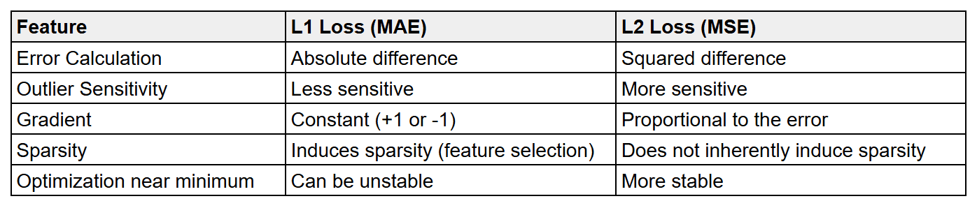
Sensitivity to Outliers: L1 loss is less sensitive to outliers because it treats all errors equally. A large error has a proportional impact on the total loss.
Gradient Behavior: The gradient of the L1 loss is constant (+1 or -1) for non-zero errors. At zero error, the gradient is undefined. This can lead to instability during optimization near the optimal solution.
Sparsity: L1 loss has a tendency to produce sparse models, meaning it can drive the weights of less important features to exactly zero. This is a desirable property for feature selection.
L2 Loss (Mean Squared Error – MSE)
L2 loss measures the average squared difference between the actual and predicted values. It is expressed as:
Where, represents the actual value for the i-th data point. represents the predicted value for the i-th data point. is the total number of data points.
Sensitivity to Outliers: L2 loss is more sensitive to outliers because it squares the errors. A large error has a disproportionately larger impact on the total loss, making the model more influenced by extreme values.
Gradient Behavior: The gradient of the L2 loss is proportional to the error (2( – )). This means that larger errors have larger gradients, which can help the optimization process converge faster when the errors are large. As the error approaches zero, the gradient also approaches zero, leading to more stable convergence near the optimal solution.
Sparsity: L2 loss does not inherently lead to sparse models. It tends to shrink the weights of all features, but rarely drives them to exactly zero.
Leave a Reply