
What is Structure from Motion (SfM), and how do deep learning models such as DUSt3R, MASt3R, and VGGT replace traditional keypoint matching and bundle adjustment pipelines?
Answer
Structure from Motion is the problem of recovering both the 3D geometry of a scene (structure) and the camera poses that observed it (motion) from a set of unordered 2D images, up to a global similarity transform. The classical solution is a long pipeline of separately engineered stages: detect keypoints, match descriptors across image pairs, reject outliers with RANSAC on an epipolar constraint, register cameras incrementally with PnP and triangulation, and finally run bundle adjustment, a sparse nonlinear least-squares refinement of all cameras and points against reprojection error. The learned replacements collapse that chain into a regression problem. DUSt3R takes two uncalibrated images and directly predicts dense pointmaps, one 3D point per pixel for both images expressed in the coordinate frame of the first camera, so depth, intrinsics, and relative pose fall out of the output instead of being estimated by geometry. MASt3R adds a dense local-feature head so the same network also emits pixel-accurate correspondences, and VGGT generalizes the idea to many views at once, returning cameras, depth maps, pointmaps, and point tracks for tens or hundreds of frames in a single forward pass with no optimization loop at inference time.
(1) What SfM Actually Solves: recover camera intrinsics and extrinsics plus scene points from images alone, with scale unobservable without an external reference. Everything downstream (MVS, SLAM, NeRF, Gaussian splatting) depends on those poses.
(2) The Classical Chain Is Brittle At Its Joints: keypoints → matching → RANSAC → incremental registration → bundle adjustment. Each stage discards information, and a failure at the front (textureless walls, repeated facades, tiny baselines) cannot be recovered later.
(3) Pointmap Regression Replaces Triangulation: DUSt3R regresses  and
 in one shared frame, so the network solves calibration, depth, and relative pose jointly instead of chaining three estimators.
(4) MASt3R Restores Pixel-Level Precision: a 24-dimensional dense descriptor head trained with an InfoNCE matching loss plus fast reciprocal matching gives sub-pixel correspondences that pure 3D regression blurs, and MASt3R-SfM builds a full reconstruction pipeline on top with no RANSAC.
(5) VGGT Removes The Optimizer: alternating frame-wise and global self-attention over all views, with camera and register tokens, yields cameras, depth, pointmaps, and tracks feed-forward in seconds. Bundle adjustment becomes an optional post-hoc refinement rather than the core algorithm.
(6) The Trade-off Is Priors Versus Guarantees: learned models succeed where geometry is degenerate (near-zero baseline, no texture, minimal overlap) but their accuracy is bounded by training data, output is up to scale, and global attention is quadratic in total token count.
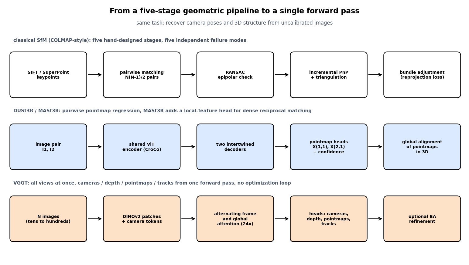
Figure 1: The same task, three levels of learned integration. The classical row has five hand-designed stages with five distinct failure modes; DUSt3R keeps only a lightweight 3D global alignment over pairwise predictions; VGGT keeps nothing optimization-based at all, and bundle adjustment survives only as an optional refinement.
The conceptual pivot is the pointmap. A depth map is defined only relative to its own camera, so combining two of them requires knowing intrinsics and relative pose first. A pointmap for image  expressed in the frame of camera 1, written
 , already lives in a shared space. Once both images are mapped into that space, the classical unknowns are read out rather than solved for: focal length comes from fitting a pinhole model to the ray field of , relative pose comes from Procrustes alignment or PnP between and camera 2’s own rays, and correspondence becomes a nearest-neighbour query in 3D rather than a descriptor comparison. That is why DUSt3R needs neither intrinsics nor an initial pose guess, and why it degrades gracefully instead of failing outright when overlap is small.
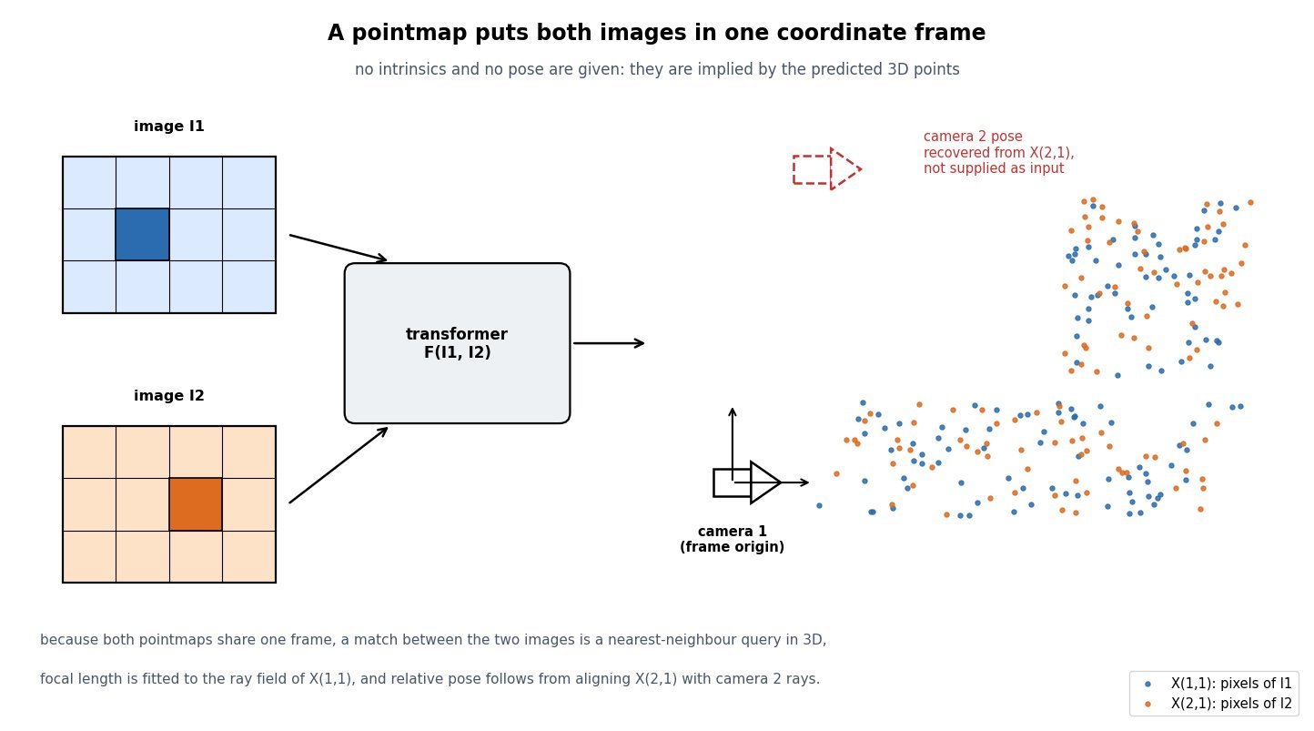
Figure 2: Both pointmaps are regressed in one coordinate frame, the frame of camera 1. Because pixels of  land directly in that frame, the relative pose is implied by the output rather than required as input, and a match between the two images is just a pair of nearby 3D points.
Classical Objective (Bundle Adjustment):


Where:
 is the total reprojection error, minimized over cameras and points jointly by Levenberg-Marquardt with a Schur-complement trick on the sparse normal equations.
- is a triangulated scene point and the 2D keypoint where camera observed it.
- is the visibility set, that is the surviving inlier matches; every match RANSAC rejected is simply absent, so the objective can only refine, never repair, the front end.
- are the intrinsics, rotation, and translation of camera , all unknown and all coupled through the same residuals.
 is the total reprojection error, minimized over cameras and points jointly by Levenberg-Marquardt with a Schur-complement trick on the sparse normal equations.
 is a triangulated scene point and
 the 2D keypoint where camera
 observed it.
 is the visibility set, that is the surviving inlier matches; every match RANSAC rejected is simply absent, so the objective can only refine, never repair, the front end.
 are the intrinsics, rotation, and translation of camera
Learned Objective (DUSt3R Pointmap Regression):


Where:
- is the transformer that consumes the raw pair with no camera parameters, built from a shared ViT encoder and two decoders that exchange information by cross-attention.
- is the pointmap of view in the frame of camera 1, so is what encodes the relative pose, and is the per-pixel confidence.
- indexes valid pixels, is the ground-truth point, and are scale normalizers (mean distance to the origin) that make the loss scale-invariant.
- weights the log-confidence regularizer, letting the network downweight sky, transparent surfaces, and non-overlapping regions instead of hallucinating them with full certainty.
- Multi-view reconstruction then optimizes a 3D alignment loss over a graph of pairwise predictions, not a reprojection loss, which is why the global step takes seconds rather than the minutes a full bundle adjustment needs.
 is the transformer that consumes the raw pair with no camera parameters, built from a shared ViT encoder and two decoders that exchange information by cross-attention.
 is the per-pixel confidence.
 is the ground-truth point, and
 are scale normalizers (mean distance to the origin) that make the loss scale-invariant.
 weights the log-confidence regularizer, letting the network downweight sky, transparent surfaces, and non-overlapping regions instead of hallucinating them with full certainty.
VGGT changes the scaling story. Instead of predicting pairs and stitching them, it patchifies all  frames with a DINOv2 backbone, appends per-frame camera tokens and register tokens, and then alternates two attention types for 24 blocks: frame-wise attention that reasons within one image, and global attention that reasons across every token of every image. The first frame’s camera token is given a distinct embedding, which is how the network fixes the output coordinate frame to camera 1 without any positional trick. Heads then decode a 9-dimensional camera parametrization (rotation quaternion, translation, field of view), a DPT depth map, a pointmap, and dense tracking features, all supervised directly.
Feed-Forward Multi-View Prediction (VGGT):


Where:
- holds camera ‘s pose and intrinsics, its depth map, its pointmap, and its tracking features, all produced in one forward pass.
- is the token count per frame at 518-pixel input with 14-pixel patches, and the total sequence length that global attention must span.
- is the model width; alternating the cheap frame-wise term with the expensive global term is what keeps hundreds of views tractable, and the quadratic global term is what eventually exhausts GPU memory.
 holds camera
 its depth map,
 its pointmap, and
 its tracking features, all produced in one forward pass.
 is the token count per frame at 518-pixel input with 14-pixel patches, and
 the total sequence length that global attention must span.
 is the model width; alternating the cheap frame-wise term with the expensive global term is what keeps hundreds of views tractable, and the quadratic global term is what eventually exhausts GPU memory.
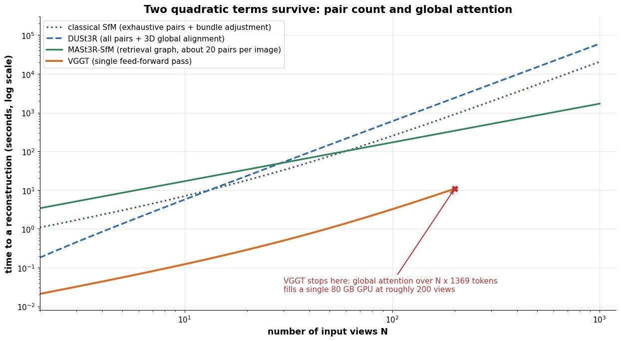
Figure 3: Feed-forward inference wins by orders of magnitude at small and medium view counts, but two quadratic terms remain in the field: exhaustive pairing (which retrieval-based graphs in MASt3R-SfM sparsify to roughly  pairs) and global attention (which sets VGGT’s memory ceiling). VGGT timings follow the published single-GPU measurements; the other curves are illustrative scaling.
| Property | Classical SfM (COLMAP-style) | DUSt3R / MASt3R | VGGT |
|---|---|---|---|
| Required input | Images, ideally with EXIF focal priors and good overlap | An uncalibrated image pair, no intrinsics, no pose init | One to hundreds of uncalibrated, unordered images |
| Core computation | Descriptor matching, RANSAC, and nonlinear least squares | Pairwise transformer inference plus a 3D global alignment | A single forward pass of alternating frame and global attention |
| Correspondence source | Explicit keypoint descriptors with geometric verification | Nearest neighbours in 3D, plus a dense descriptor head in MASt3R | A tracking head over global features, no matching stage |
| Scaling in views | Quadratic pairing, plus repeated bundle adjustment as views register | Quadratic in pairs unless a retrieval graph sparsifies it | Quadratic in total tokens, memory-bound rather than time-bound |
| Dominant failure mode | Hard failure on textureless, repetitive, or low-baseline input | Drift when many pairwise predictions must be fused | Out-of-distribution scenes and a hard memory ceiling on view count |
| Metric scale | Up to scale unless a known baseline or GPS is supplied | Up to scale by construction (scale-normalized loss) | Up to scale, with scale partly inherited from training priors |
Leave a Reply