Interview for Machine Learning

Tag: Transformer

DL0067 BERT VS GPT Pretraining
How does BERT’s pre-training objective differ from GPT’s?
Answer
BERT is trained primarily with masked language modeling: selected input tokens are corrupted, and a bidirectional encoder predicts the original tokens from visible context on both sides. GPT uses causal language modeling: a decoder predicts each next token using only earlier tokens, enforced by a triangular attention mask. MLM supplies loss only at selected positions and creates a corruption mismatch between pre-training and ordinary inputs, whereas causal modeling supplies a target at nearly every position and matches left-to-right generation. Original BERT also used next sentence prediction, while standard GPT pre-training relies on the autoregressive token objective rather than NSP.

Figure 1: BERT reconstructs selected corrupted tokens from two-sided context, while GPT predicts the next token at every step from a left-only prefix.
(1) Context Visibility: BERT’s visible tokens attend bidirectionally; GPT position $t$ cannot attend to positions later than $t$ .
(2) Prediction Targets: BERT reconstructs a selected masked subset, while GPT shifts the sequence and predicts the next token at each usable position.
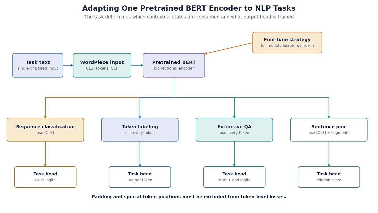
(3) Downstream Bias: BERT naturally supports full-context understanding, whereas GPT’s objective directly trains open-ended autoregressive generation; either family can be adapted beyond that bias.
Mathematical Formulation:
$\mathcal{L}_{\mathrm{BERT}}=-\sum_{i\in\mathcal{M}}\log p(x_i\mid x_{\setminus\mathcal{M}})$
$\mathcal{L}_{\mathrm{GPT}}=-\sum_{t=1}^{T}\log p(x_t\mid x_{1:t-1})$
Where:
$\mathcal{L}_{\mathrm{BERT}}$ and $\mathcal{L}_{\mathrm{GPT}}$ are the masked and causal language-modeling losses.
$\mathcal{M}$ is BERT’s selected target set and $i\in\mathcal{M}$ indexes one target token $x_i$ .
$x_{\setminus\mathcal{M}}$ denotes BERT’s visible corrupted context outside the selected targets, and $p(x_i\mid x_{\setminus\mathcal{M}})$ is the reconstruction probability.
$t\in\{1,\ldots,T\}$ indexes a GPT target position, $T$ is sequence length, and $x_{1:t-1}$ is the preceding token prefix.
$p(x_t\mid x_{1:t-1})$ is the next-token probability and $\log$ converts each probability into a log-likelihood term.

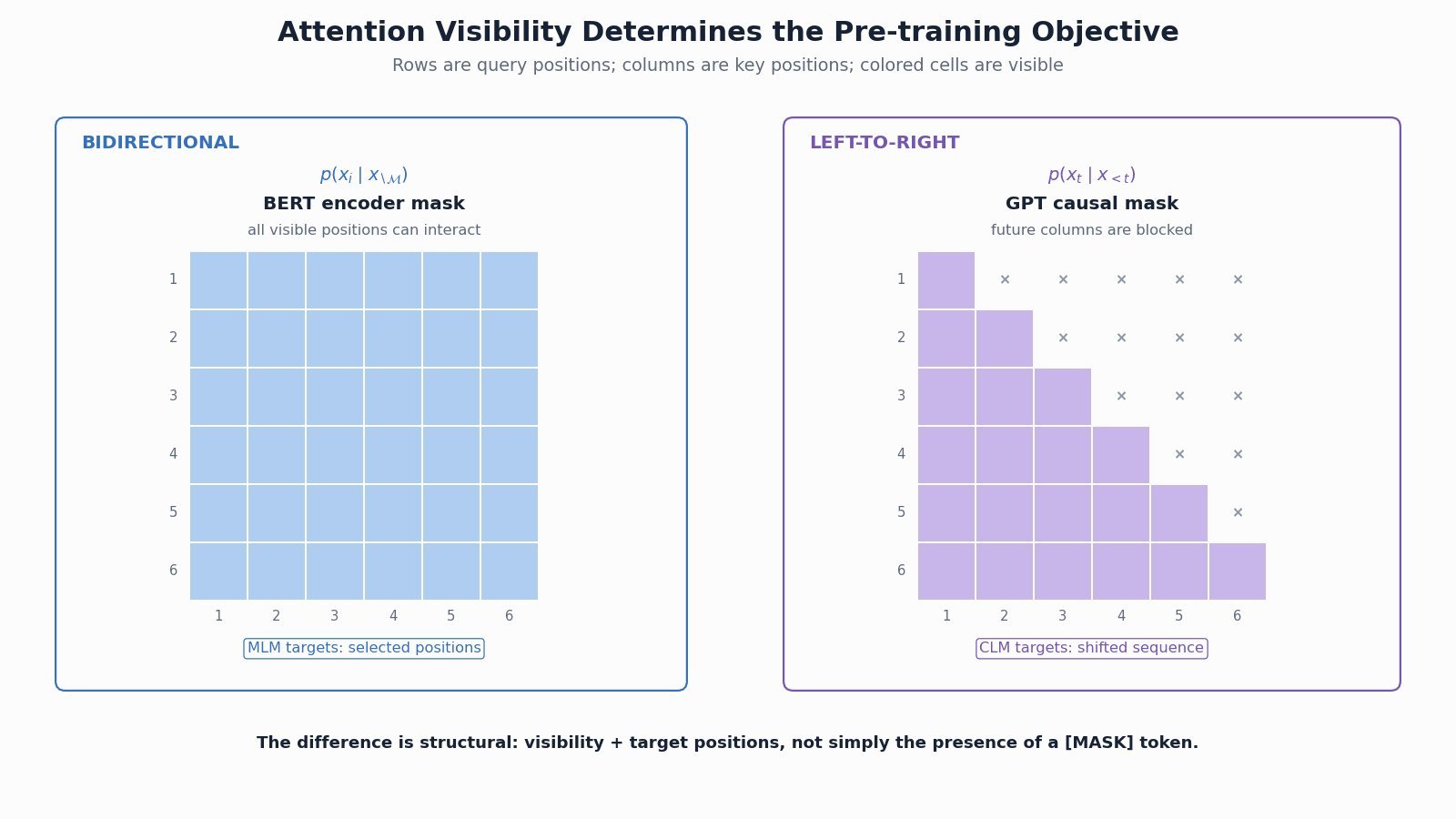
Figure 2: Attention visibility explains the objective difference: BERT uses a full visible-context matrix, while GPT uses a lower-triangular causal matrix.
Login to view more content
July 20, 2026
DL0066 BERT
What is BERT and how is it used in NLP tasks?
Answer
BERT is a Transformer encoder pretrained to build bidirectional contextual representations of text. Its input combines token, segment, and positional embeddings, and every encoder layer lets each unmasked token attend to context on both sides. Original BERT is pretrained with masked language modeling and next sentence prediction, then adapted by adding a small task head and fine-tuning the whole model or using its representations. The [CLS] output supports sequence-level tasks, token outputs support tagging, and paired start/end scores support extractive question answering.

Figure 1: BERT combines token, segment, and position embeddings, processes them with bidirectional encoder layers, and exposes contextual outputs.
(1) Bidirectional Encoder: Unlike a causal decoder, BERT‘s self-attention normally uses both left and right context for every visible input token.
(2) Pre-Training: Original BERT predicts selected masked tokens and also trains an NSP classifier; later BERT-family models often modify or remove NSP.
(3) Task Adaptation: A lightweight output head maps contextual states to sequence labels, token labels, sentence-pair scores, or answer spans.

Figure 2: The same pretrained encoder can be adapted with small heads that consume either [CLS], every token state, or start/end span scores.
Mathematical Formulation:
$H=\mathrm{Encoder}(E_{\mathrm{token}}+E_{\mathrm{segment}}+E_{\mathrm{position}})$
$\mathcal{L}_{\mathrm{MLM}}=-\sum_{i\in\mathcal{M}}\log p(x_i\mid x_{\setminus\mathcal{M}})$
Where:
$E_{\mathrm{token}}$ , $E_{\mathrm{segment}}$ , and $E_{\mathrm{position}}$ are token, segment, and positional embedding matrices for the input sequence.
$\mathrm{Encoder}$ is the bidirectional Transformer stack and $H$ contains one contextual vector per input position.
$\mathcal{L}_{\mathrm{MLM}}$ is masked-language-modeling loss and $\mathcal{M}$ is the selected set of prediction positions.
$i\in\mathcal{M}$ indexes one selected target, $x_i$ is its original token, and $x_{\setminus\mathcal{M}}$ denotes the visible corrupted context outside the selected targets.
$p(x_i\mid x_{\setminus\mathcal{M}})$ is the model probability assigned to the original target token given visible context.
Login to view more content
July 20, 2026
DL0063 Transformer Variable Length Sequences
How does the Transformer handle variable-length sequences?
Answer
A Transformer can process different sequence lengths because self-attention is defined over whatever number of tokens is supplied, up to the model’s context limit. For efficient batching, implementations usually pad sequences to a common length or group examples of similar lengths, then apply a padding mask so valid queries cannot attend to padded keys and values. Decoder-style models also add a causal mask that blocks future positions, while positional encodings identify token order within each sequence. Padded query outputs and losses must be ignored, and computation still scales with the padded batch length rather than only the number of valid tokens.
(1) Batch Construction: Sequences are dynamically padded to the longest item in a batch, bucketed by length, or packed by specialized kernels to reduce wasted work.
(2) Attention Masking: A key-padding mask removes padded keys and values from attention; causal models combine it with a triangular future mask.
(3) Length Boundary: Variable length does not mean unlimited length: positional support, memory, and the configured context window impose a maximum.

Figure 1: Unequal token sequences become a rectangular batch; masking separates valid context, padding, and future positions.
Mathematical Formulation:
$\mathrm{Attention}(Q,K,V)=\mathrm{softmax}\!\left(\frac{QK^\top}{\sqrt{d_k}}+M_{\mathrm{pad}}+M_{\mathrm{causal}}\right)V$
$M_{ij}\in\{0,-\infty\}$
Where:
$Q$ , $K$ , and $V$ are query, key, and value matrices, and $d_k$ is the key width used for score scaling.
$M_{\mathrm{pad}}$ assigns $-\infty$ to padded key positions so their softmax probabilities become zero.
$M_{\mathrm{causal}}$ assigns $-\infty$ when key index $j$ is later than query index $i$ ; encoder-only models normally omit this mask.
$M_{ij}$ denotes one combined mask entry and is either $0$ for an allowed connection or $-\infty$ for a blocked connection.
$B$ is batch size and $L_{max}$ is padded sequence length, giving a dense token tensor of shape $B\times L_{max}$ .

Figure 2: A practical variable-length pipeline: tokenize, bucket or pad, build masks, run attention, then ignore padded outputs or continue autoregressive generation.
Login to view more content
July 20, 2026
DL0061 Channel and Spatial Attention
Explain channel attention and spatial attention in CNNs. What information does each mechanism model?
Answer
Channel attention learns which feature channels are important, answering what semantic responses should be emphasized. It compresses spatial dimensions into channel descriptors, transforms them with a small gating network, and multiplies the resulting weights into the feature tensor. Spatial attention learns where informative regions occur by compressing or projecting the channel dimension and producing an $H\times W$ mask. Modules such as SE use channel attention, while CBAM applies channel attention followed by spatial attention to refine both feature type and location.

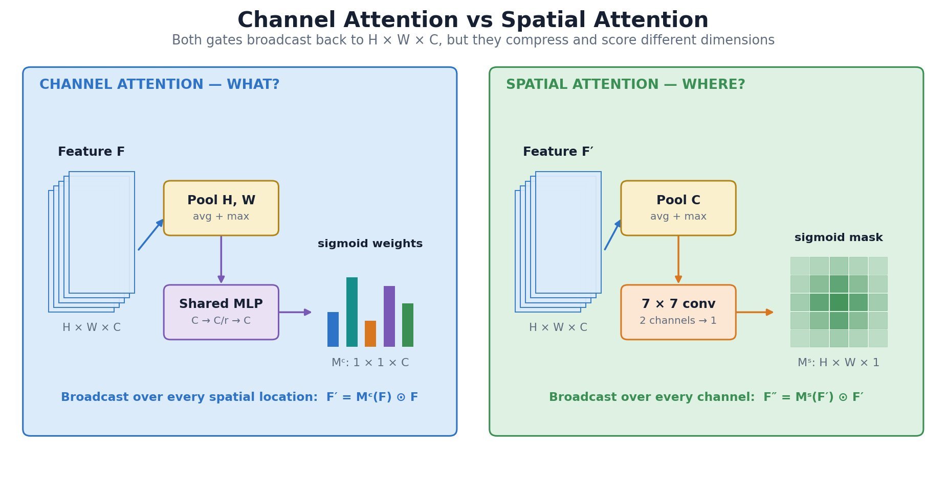
Figure 1: Parallel tensor-shape explanation of what channel attention selects and where spatial attention focuses.
(1) Channel Gate: Global pooling summarizes each channel; an MLP or 1D convolution captures inter-channel dependence and outputs $C$ multiplicative weights.
(2) Spatial Gate: Average/max pooling or learned projection across channels produces spatial descriptors that a convolution maps to one $H\times W$ attention mask.
(3) Residual Placement: Attention usually modulates an existing feature tensor and is often inserted inside a residual block; sigmoid gates reweight rather than replace the underlying features.

Figure 2: CBAM data flow from input feature through channel gating, spatial gating, residual refinement, and output.
Mathematical Formulation:
$M_c(F)=\sigma\!\left(\mathrm{MLP}(\mathrm{AvgPool}_{hw}(F))+\mathrm{MLP}(\mathrm{MaxPool}_{hw}(F))\right)$
$M_s(F)=\sigma\!\left(f^{7\times7}([\mathrm{AvgPool}_{c}(F);\mathrm{MaxPool}_{c}(F)])\right)$
Where:
$F\in\mathbb{R}^{H\times W\times C}$ is the input feature map with height $H$ , width $W$ , and $C$ channels.
$M_c(F)\in\mathbb{R}^{1\times1\times C}$ is the channel mask; spatial average/max pooling and the shared $\mathrm{MLP}$ produce channel logits.
$M_s(F)\in\mathbb{R}^{H\times W\times1}$ is the spatial mask; channel pooling outputs are concatenated by $[\,;\,]$ and filtered by $f^{7\times7}$ .
$\sigma$ is the sigmoid function; $M_c$ broadcasts over $H,W$ , while $M_s$ broadcasts over $C$ .
Login to view more content
July 20, 2026
DL0056 FlashAttention
Explain FlashAttention. Why can it compute exact attention faster while using less memory?
Answer
FlashAttention is an exact, IO-aware implementation of scaled dot-product attention. Instead of materializing the full $N\times N$ score and probability matrices in high-bandwidth memory (HBM), it loads blocks of $Q$ , $K$ , and $V$ into fast on-chip SRAM, computes attention block by block, and maintains online softmax statistics. Tiling reduces expensive HBM reads and writes, while recomputation during the backward pass can be cheaper than storing large intermediates. The mathematical result matches standard attention up to normal floating-point differences; the speedup comes from changing the execution schedule, not from approximating attention.

Figure 1: IO comparison showing why avoiding N×N intermediate writes makes FlashAttention faster and more memory efficient.
(1) IO Awareness: The kernel is organized around the GPU memory hierarchy so most score computation and softmax updates happen in SRAM.
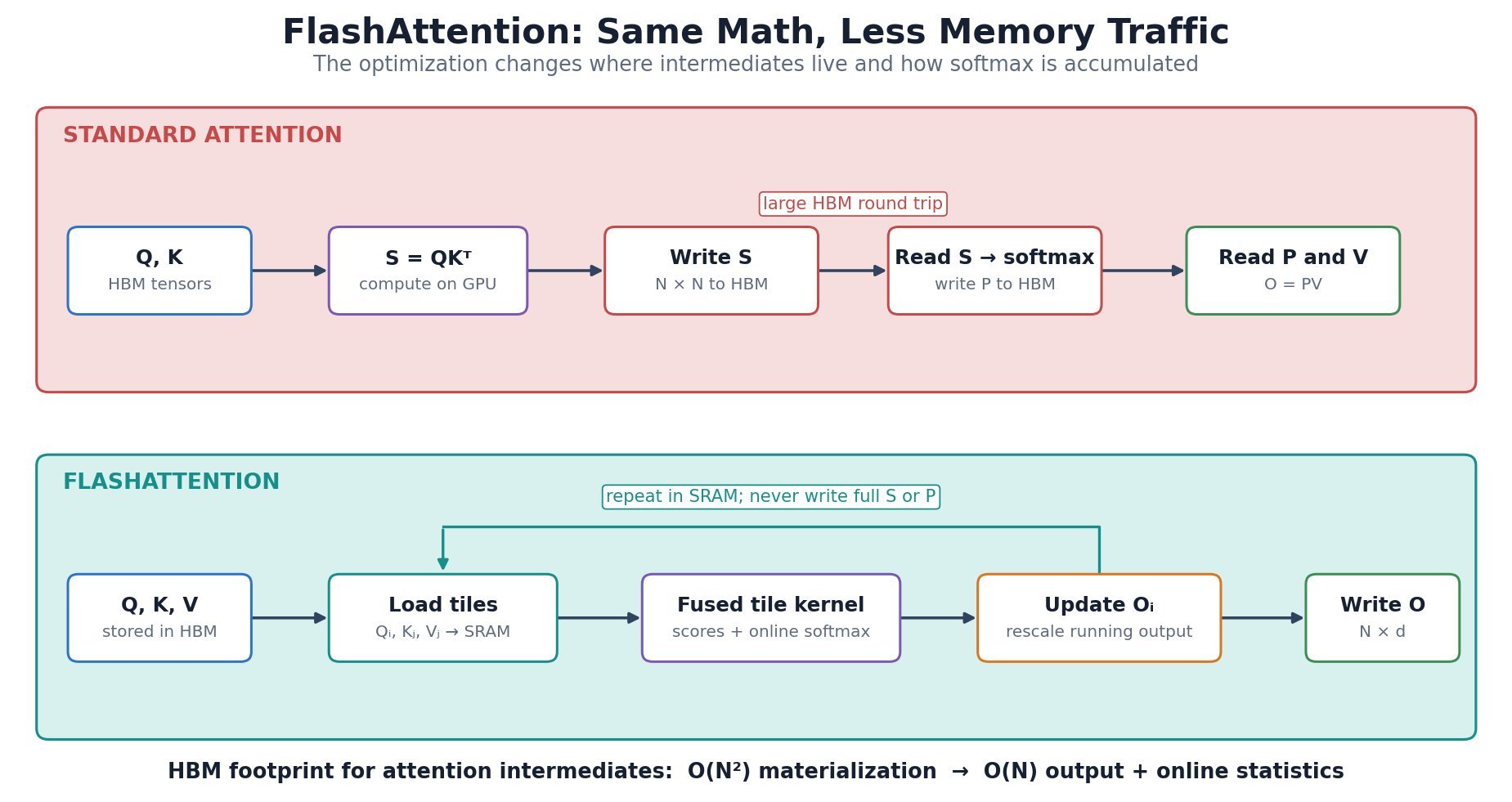
(2) Online Softmax: A running row maximum and normalization sum allow each $K,V$ tile to update the output without retaining previous score blocks.
(3) Exact Result: All query-key interactions are evaluated; causal masking, dropout, and backward gradients are fused into specialized kernels rather than approximated.
Mathematical Formulation:
$m_i^{(t)}=\max\!\left(m_i^{(t-1)},\max_j S_{ij}^{(t)}\right)$
$\ell_i^{(t)}=e^{m_i^{(t-1)}-m_i^{(t)}}\ell_i^{(t-1)}+\sum_j e^{S_{ij}^{(t)}-m_i^{(t)}}$
Where:
$t$ indexes key/value tiles, $i$ indexes a query row, and $j$ indexes keys inside tile $t$ .
$S_{ij}^{(t)}=Q_iK_j^T/\sqrt d$ is the scaled score between query row $Q_i$ and key row $K_j$ , with head width $d$ .
$m_i^{(t)}$ is the running row maximum after tile $t$ , initialized with $m_i^{(0)}=-\infty$ .
$\ell_i^{(t)}$ is the running softmax denominator, initialized with $\ell_i^{(0)}=0$ ; the exponential factors rescale earlier partial sums when the maximum changes.

Figure 2: Blockwise FlashAttention loop with running maximum, normalization, output rescaling, and final HBM write.
Login to view more content
July 20, 2026
DL0055 Vision Transformer
Explain the Vision Transformer (ViT). How does it convert an image into a class prediction?
Answer
A Vision Transformer converts an image into a sequence of fixed-size patch tokens and processes them with a Transformer encoder. A learned class token is prepended, positional embeddings preserve patch order, and global self-attention lets every patch exchange information with every other patch. After the encoder stack, the class-token representation is passed to a prediction head. Compared with a CNN, a ViT has weaker built-in locality and translation bias, but it can model long-range interactions directly and scales effectively with data and compute.

Figure 1: ViT architecture with tensor shapes, patch tokenization, the Transformer encoder stack, and the classification path.
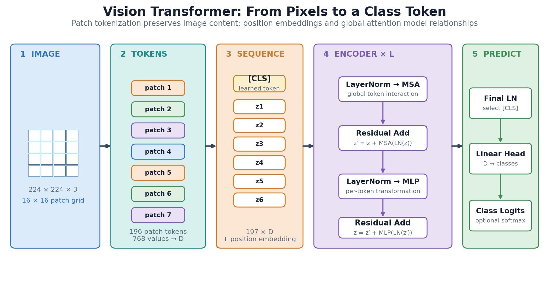
(1) Tokenization: An image of shape $H\times W\times C$ is divided into $N=(H/P)(W/P)$ non-overlapping $P\times P$ patches; each flattened patch is projected to width $D$ .
(2) Global Context: Multi-head self-attention mixes information across all patch positions, while residual connections and MLP sublayers refine each token.
(3) Classification: A learned [CLS] token aggregates evidence across the encoder stack; its final state is normalized and mapped to class logits.

Figure 2: ViT inference flow from image validation and patch embedding to encoder processing and class prediction.
Mathematical Formulation:
$z_0=[x_{\mathrm{cls}};x_p^1E;x_p^2E;\ldots;x_p^NE]+E_{\mathrm{pos}}$
$\mathrm{Attention}(Q,K,V)=\mathrm{softmax}\!\left(\frac{QK^T}{\sqrt{d_h}}\right)V$
Where:
$z_0$ is the initial token sequence supplied to the Transformer encoder.
$x_{\mathrm{cls}}$ is the learned class token, and $x_p^i$ is flattened image patch $i$ .
$E\in\mathbb{R}^{P^2C\times D}$ projects each $P\times P\times C$ patch to width $D$ , while $E_{\mathrm{pos}}$ supplies positional embeddings.
$N=(H/P)(W/P)$ is the patch count for an image of height $H$ , width $W$ , and channel count $C$ .
$Q$ , $K$ , and $V$ are query, key, and value matrices; $d_h$ is the per-head query/key width.
Login to view more content
July 20, 2026
DL0054 Deformable Attention
What is Deformable Attention and how does it reduce computational complexity for object detection tasks?
Answer
Deformable Attention is a sparse attention mechanism that learns dynamic sampling locations instead of attending to all spatial positions uniformly. It uses learned 2D offsets from reference points to sample only the most relevant features, reducing complexity from $O(N^2)$ to $O(NK)$ where K is a small constant (typically 4). This makes it ideal for high-resolution feature maps in object detection where full attention is computationally prohibitive — for a 1024×1024 feature map, standard attention requires ~1M operations per head while deformable attention needs only ~4K.

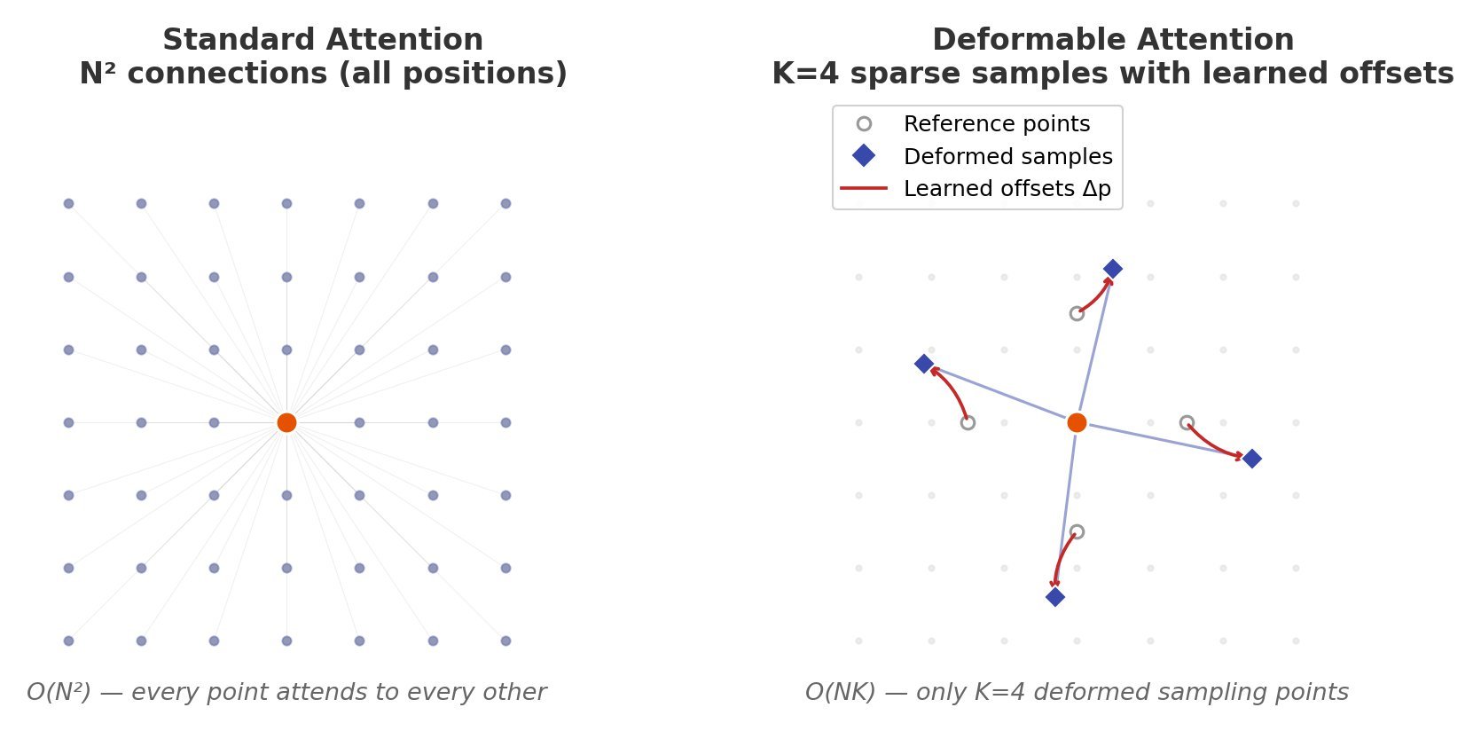
Figure 1: Deformable attention learns K=4 sampling offsets per query point instead of dense N×N attention
(1) Sparse Sampling: Instead of computing attention over all $N \times N$ positions, deformable attention samples only K reference points per query, typically K=4 or 8, reducing the key-value set from N to K.
(2) Learned Offsets: The model predicts $\Delta p_{mk}$ offsets from each reference point $p_k$ using a lightweight linear layer on query features, requiring only $O(NC)$ additional computation where C is channel dimension.
(3) Bilinear Interpolation: When offsets point to non-integer locations, bilinear interpolation computes feature values from the 4 nearest pixels, enabling sub-pixel precision sampling without modifying the feature map.

Figure 2: Complexity comparison shows O(NK) grows linearly while O(N²) becomes prohibitive for large feature maps
Mathematical Formulation:
$y(p) = \sum_{m=1}^{M} W_m \left[ \sum_{k=1}^{K} A_{mk} \cdot W_m' x(p + p_k + \Delta p_{mk}) \right]$
Where:
$p$ is the reference position (query location on the feature map)
$M$ is the number of attention heads
$K$ is the number of sampled keys per head (typically 4)
$p_k$ are fixed reference offsets (uniformly initialized)
$\Delta p_{mk}$ are learned deformable offsets (2D, predicted per head per key)
$A_{mk}$ is the attention weight (normalized, not from softmax over all positions)
$W_m, W_m'$ are projection matrices for each head
The offsets $\Delta p_{mk}$ are predicted by a linear projection from query features: $\Delta p_{mk} = W_\text{offset} \cdot q_m(p)$ , where $W_\text{offset} \in \mathbb{R}^{C \times 2K}$ . The attention weights $A_{mk}$ are computed via a separate softmax over only K elements, not the full N positions. In Deformable DETR, multi-scale deformable attention extends this to sample across multiple feature map resolutions simultaneously, enabling the model to capture both small and large objects efficiently.
Login to view more content
July 13, 2026
DL0053 Gated Attention
What is Gated Attention and how does it improve transformer architectures over standard scaled dot-product attention?
Answer
Gated Attention (arXiv:2505.06708) applies a head-specific sigmoid gate after Scaled Dot-Product Attention (SDPA) to dynamically modulate attention output. Unlike standard attention where all heads contribute equally, gated attention introduces query-dependent sparse gating that suppresses irrelevant heads and activates only salient ones. This mitigates the attention sink problem where standard transformers concentrate disproportionate attention on the first few tokens, and enhances long-context extrapolation by maintaining diverse attention patterns across sequence lengths.

Figure 1: Gated attention applies a head-specific sigmoid gate after SDPA to modulate attention output before the residual connection
(1) Post-SDPA Gating: The gate is applied after SDPA computation, not before — each attention head $h_i$ is multiplied by a sigmoid gate $g_i = \sigma(W_g \cdot q_i)$ where $W_g$ is a head-specific projection.
(2) Sparsity Induction: The sigmoid gate produces values in $[0, 1]$ , and empirical measurements show mean gate activation of ~0.116, meaning most heads are heavily suppressed — introducing beneficial sparsity without hard pruning.
(3) Attention Sink Mitigation: Standard attention allocates ~46.7% of attention mass to the first token; gated attention reduces this to ~4.8%, distributing attention more uniformly across tokens.

Figure 2: Gate activation distribution across 8 attention heads shows heavy suppression (mean ~0.116) with sparse high-activation regions
Mathematical Formulation:
$\text{GatedAttn}(Q, K, V) = \text{Concat}(g_1 \odot h_1, \ldots, g_H \odot h_H) W_O$
$g_i = \sigma(W_g^{(i)} \cdot q_i + b_g^{(i)})$
Where:
$h_i = \text{SDPA}(q_i, k_i, v_i)$ is the output of the $i$ -th attention head
$g_i \in [0, 1]$ is the head-specific gate score
$W_g^{(i)} \in \mathbb{R}^{d_k \times 1}$ is a learned projection from query to scalar gate
$\sigma$ is the sigmoid function
$\odot$ denotes element-wise multiplication
$W_O$ is the standard output projection
The gate projection $W_g^{(i)}$ adds only $O(d_k)$ parameters per head — a negligible overhead of ~0.1% of total model parameters — yet significantly improves long-context performance. On the RULER benchmark at 128K context length, gated attention improves needle-in-haystack retrieval accuracy from ~72% to ~94% compared to standard attention.
Login to view more content
July 13, 2026
DL0052 Rotary Positional Embedding
What is Rotary Positional Embedding (RoPE)?
Answer
Rotary Positional Embedding (RoPE) is a positional encoding method that rotates query and key vectors in multi‑head attention by position‑dependent angles. This rotation naturally encodes relative positional information, improves generalization to longer contexts, and avoids the limitations of fixed or learned absolute positional embeddings. It is used in GPT-NeoX, LLaMA, PaLM, Qwen, etc.
It has below charactretidstics:
(1) Relative position encoding method for Transformers
(2) Applies rotation to query (Q) and key (K) vectors using position-dependent angles
(3) Encodes position via geometry, not by adding vectors
(4) Preserves relative distance naturally in dot-product attention
(5) Extrapolates well to longer sequences than the training length
RoPE rotates each 2D pair of hidden dimensions:
$f(x, m)=\begin{pmatrix}\cos(m\theta) & -\sin(m\theta) \\ \sin(m\theta) & \cos(m\theta)\end{pmatrix}\begin{pmatrix}x_1 \\x_2\end{pmatrix}$
Where:
$m$ represents the absolute position of the token in the sequence.
$\theta$ represents the base frequency/rotation angle.
$x_1, x_2$ represent the components of the embedding vector.
The below plot visualizes how RoPE makes attention decay smoothly with relative distance, while standard sinusoidal PE reflects absolute position similarity.
Login to view more content
January 2, 2026
DL0045 Dimension in FFN
In Transformers, why does the feed-forward network expand the hidden dimension (e.g., $d_{\text{model}}$ → $4 d_{\text{model}}$ ) before reducing it back?
Answer
The feed-forward network in Transformers expands the hidden dimension (e.g., $d_{\text{model}} \to 4 \cdot d_{\text{model}}$ ) to enhance the model’s ability to learn complex, non-linear feature interactions, then reduces it back to maintain compatibility with other layers. This design acts as a bottleneck, balancing expressiveness and efficiency, and has been empirically shown to boost performance in large-scale models.
(1) Extra Capacity: Expanding from $d_{\text{model}}$ to $4d_{\text{model}}$ allows the FFN to capture richer nonlinear transformations.
(2) Non‑linear mixing: The intermediate expansion allows the activation function (ReLU, GeLU, SwiGLU, etc.) to operate in a richer space, capturing more complex patterns.
(3) Projection back ensures compatibility: Reducing the dimension back to $d_{\text{model}}$ ensures compatibility with the subsequent layers. It ensures residual connection compatibility and uniformity across layers.
The equation and the figure below show the architecture of FFN:
$\text{FFN}(x) = W_2 \sigma(W_1 x + b_1) + b_2$
Where:
$x \in \mathbb{R}^{d_{\text{model}}}$ is the input vector.
$W_1 \in \mathbb{R}^{4d_{\text{model}} \times d_{\text{model}}}$ expands the dimension.
$\sigma$ is a non-linear activation (e.g., ReLU/GELU).
$W_2 \in \mathbb{R}^{d_{\text{model}} \times 4d_{\text{model}}}$ projects back down.
Login to view more content
September 24, 2025