Author: admin

  • ML0007 Dropout

    What is dropout in neural network training?

    Answer

    Dropout is a regularization technique used during neural network training to prevent overfitting. At each training step, a fraction of neurons (and their connections) are randomly “dropped out”, meaning their activations are set to zero. This forces the network to learn more robust features, because it cannot rely on any single neuron; instead it learns distributed representations, effectively training an ensemble of many smaller sub-networks that share weights. At inference time every neuron is active, so the model uses all learned features without randomness. To bridge the train/inference gap, inverted dropout scales the active neurons by 1/(1-p) during training so no adjustment is needed at inference; the alternative standard dropout scales the weights by (1-p) at inference instead.

    (1) Mechanism: Randomly zero a fraction p of activations per training step; the dropped set changes every step.
    (2) Why It Works: Prevents co-adaptation of neurons and approximates training an exponentially large ensemble of sub-networks.
    (3) Training vs Inference: Inference uses the full network; activations are rescaled (during training with inverted dropout, or at inference with standard dropout) so expected magnitudes match.

    Full network versus the same network with randomly dropped neurons

    Figure 1: Left: the full network. Right: one training step with dropout: grayed, crossed-out neurons are zeroed, forcing the remaining sub-network to carry the prediction.

    Mathematical Formulation:
    \tilde{h}_i = \frac{m_i}{1-p} \cdot h_i
    m_i \sim \mathrm{Bernoulli}(1-p)

    Where:

    • \tilde{h}_i is the scaled activation of neuron i actually passed to the next layer during training.
    • h_i is the original activation of neuron i, and i indexes the neurons in a layer.
    • m_i is the binary dropout mask: 1 keeps the neuron, 0 drops it.
    • p is the drop probability; 1-p is the keep probability, and dividing by it is the inverted-dropout scaling that keeps \mathbb{E}[\tilde{h}_i] = h_i.
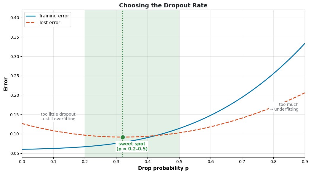
    Training and test error versus dropout rate with a sweet spot region

    Figure 2: Choosing the drop probability p: too little dropout leaves overfitting, too much underfits; the test-error minimum is the sweet spot (typically p around 0.2–0.5).


    Login to view more content
  • ML0006 Cross-Validation

    What are the common cross-validation techniques?

    Answer

    Cross-validation is a statistical method used to evaluate the performance and generalizability of a model by rotating which part of the data serves as the validation set, so every sample is used for both training and validation. The most common technique is k-Fold Cross-Validation: the data is divided into k equal folds, the model is trained k times, each time on k-1 folds with the remaining fold held out, and the final score is the average over all k runs. Leave-One-Out Cross-Validation (LOOCV) is the special case where k equals the number of data points. Stratified k-Fold preserves the class distribution inside every fold, which matters for imbalanced datasets. Time Series Cross-Validation builds folds that respect temporal order, preventing future data from leaking into training.

    (1) Core Idea: Rotate the validation fold and average the scores, giving a more reliable estimate than a single train/validation split.
    (2) Choosing The Variant: k=5 or 10 is the default, LOOCV suits tiny datasets, stratified folds suit class imbalance, and TSCV is mandatory for sequential data.
    (3) Why It Matters: Every sample gets validated on, so the estimate has lower variance and uses all the data, at the cost of training k times.

    Four cross-validation schemes: k-fold, LOOCV, stratified k-fold, and time series CV

    Figure 1: Four cross-validation schemes. Orange blocks are validation folds: they rotate (k-fold), shrink to one sample (LOOCV), keep class ratios (stratified), or move forward in time (TSCV).

    Mathematical Formulation:
    \mathrm{CV}_k = \frac{1}{k}\sum_{i=1}^{k}\mathcal{E}_i
    \mathcal{E}_i = \mathcal{L}\big(\hat{f}_{-i}, D_i\big)

    Where:

    • \mathrm{CV}_k is the cross-validation score, the average error across all k folds.
    • \mathcal{E}_i is the validation error on fold i, and i\in\{1,\ldots,k\} indexes the folds.
    • \hat{f}_{-i} is the model trained on all folds except fold i, and D_i is the held-out fold.
    • \mathcal{L} is the evaluation loss or metric (e.g., error rate, log-loss).

    Login to view more content
  • ML0005 Discriminative and Generative

    What are the differences between discriminative and generative models?

    Answer

    Discriminative models learn to draw a boundary between classes: they model the conditional probability P(y \mid x) directly, mapping features x to labels y without modeling how the data was generated. Examples include logistic regression, support vector machines, and neural network classifiers. Generative models instead estimate the joint probability P(x, y) (via P(x \mid y) and P(y)), capturing how the data itself is generated, and then use Bayes’ theorem to derive P(y \mid x) for classification. Examples include Naive Bayes, hidden Markov models, VAEs, and GANs. Because generative models learn the data distribution, they can also sample new data; discriminative models can only separate existing classes.

    (1) Modeling Target: Discriminative models learn P(y \mid x) directly; generative models learn P(x, y) or P(x \mid y) P(y).
    (2) Decision Mechanism: Discriminative models find a decision boundary; generative models compare class-conditional densities through Bayes’ rule.
    (3) Capabilities: Discriminative models only classify; generative models can also generate samples, handle missing features, and score outliers.

    Discriminative model separates classes with a boundary; generative model fits a distribution per class

    Figure 1: Left: a discriminative model cares only about the boundary between classes. Right: a generative model fits a distribution to each class, capturing how the data itself looks.

    Mathematical Formulation:
    \text{discriminative:} \quad \hat{y} = \arg\max_y \, P(y \mid x)
    \text{generative:} \quad P(y \mid x) = \frac{P(x \mid y)\, P(y)}{P(x)}

    Where:

    • \hat{y} is the predicted label and y ranges over the class set for input x.
    • P(y \mid x) is the posterior, the quantity a discriminative model learns directly.
    • P(x \mid y) is the class-conditional likelihood (how data of class y looks) and P(y) the class prior; together they define the joint P(x, y) a generative model learns.
    • P(x) is the evidence normalizer, computable as \sum_y P(x \mid y) P(y) over all classes.

    Login to view more content
  • ML0004 Underfitting

    What is underfitting, how do you recognize it, and how can you fix it?

    Answer

    Underfitting occurs when a model is too simple to capture the underlying patterns in the data, so it performs poorly on both the training data and new, unseen data: it has not even learned the training set. An underfit model exhibits high bias and low variance: its predictions are consistently wrong in the same way, regardless of the particular training sample. Common causes are an overly simple model, inadequate training (stopped too early), over-regularization, and poor feature selection. The fixes mirror the causes: increase model complexity, train longer, reduce regularization, and engineer more informative features.

    (1) Definition: The model lacks the capacity to fit the signal, so error stays high on training and test data alike.
    (2) Recognition: High training error is the key signature; contrast with overfitting, where training error is low and only validation error suffers.
    (3) Fixes: Add capacity (more layers, higher-degree features), train longer, weaken regularization, and improve the feature set.

    Three fits to the same data: underfit line, good low-degree fit, and overfit high-degree curve

    Figure 1: The same data fitted three ways. The underfit line misses the pattern entirely; the good fit follows the trend; the overfit curve chases every noisy point.

    Mathematical Formulation:
    \mathrm{Err}(x_0) = \mathrm{Bias}^2\big(\hat{f}(x_0)\big) + \mathrm{Var}\big(\hat{f}(x_0)\big) + \sigma^2
    \text{underfitting} \;\Rightarrow\; \mathrm{Bias}^2 \text{ dominates the total error}

    Where:

    • \mathrm{Err}(x_0) is the expected prediction error of the model \hat{f} at a new point x_0.
    • \mathrm{Bias}^2 measures how far the average prediction sits from the truth: the term that dominates when a model underfits.
    • \mathrm{Var} measures how much the prediction swings across different training sets: the term that dominates in overfitting.
    • \sigma^2 is the irreducible noise in the data, which no model can remove.

    Login to view more content
  • ML0003 Overfitting

    What is overfitting and how to avoid overfitting?

    Answer

    Overfitting happens when a model learns the training data too well (including its noise and outliers) and as a result performs poorly on new, unseen data. The model becomes too specialized to the training set and fails to generalize. The telltale sign is a growing generalization gap: training loss keeps falling while validation loss turns back up. To avoid overfitting: simplify the model, get more data or use data augmentation, apply regularization (L1/L2), validate frequently with early stopping, and for neural networks use dropout.

    (1) Definition: The model memorizes noise as if it were signal, so training error keeps dropping while test error rises.
    (2) Detection: Watch the train/validation loss gap and use cross-validation: wildly varying performance across folds indicates overfitting.
    (3) Remedies: More or augmented data, L1/L2 regularization, dropout, early stopping, or a smaller model; all reduce effective capacity or expose the model to more variation.

    Training loss keeps decreasing while validation loss turns upward, with an early stopping marker

    Figure 1: The validation loss minimum marks the ideal stopping point; training past it widens the generalization gap; that widening is overfitting.

    Mathematical Formulation:
    \mathcal{L}_{\mathrm{reg}}(\theta) = \mathcal{L}(\theta) + \lambda \lVert \theta \rVert_2^2
    \mathrm{gap} = \mathcal{L}_{\mathrm{val}}(\theta) - \mathcal{L}_{\mathrm{train}}(\theta)

    Where:

    • \mathcal{L}(\theta) is the original training loss over parameters \theta.
    • \lambda is the regularization strength; larger values shrink the weights \theta toward zero, trading training fit for generalization.
    • \lVert \theta \rVert_2^2 is the squared L2 norm of the weights (weight decay); an L1 penalty \lVert \theta \rVert_1 instead drives weights to exactly zero.
    • \mathcal{L}_{\mathrm{val}} and \mathcal{L}_{\mathrm{train}} are validation and training loss; a small, stable gap indicates good generalization.
    Bias-variance tradeoff: total error is U-shaped over model complexity

    Figure 2: Why the remedies work: they move the model left along the complexity axis, out of the high-variance region and back toward the total-error minimum.


    Login to view more content
  • ML0002 Machine Learning Type

    What is the difference between supervised learning and unsupervised learning?

    Answer

    Supervised learning trains on labeled data (every example comes with a target output) and learns a mapping that predicts the label of new, unseen inputs. Unsupervised learning works on unlabeled data and instead discovers hidden structure in the inputs themselves, such as clusters or low-dimensional representations. The practical difference is the supervision signal: supervised models are corrected against known answers during training, while unsupervised models optimize an intrinsic objective like reconstruction error or cluster compactness. Supervised learning covers classification and regression; unsupervised learning covers clustering and dimensionality reduction.

    (1) Data Requirement: Supervised needs input–label pairs (x_i, y_i); unsupervised needs only inputs x_i, which are far cheaper to collect.
    (2) Learning Objective: Supervised minimizes prediction error against the labels; unsupervised optimizes structure objectives such as cluster compactness or reconstruction loss.
    (3) Typical Tasks: Classification and regression for supervised; clustering, dimensionality reduction, and density estimation for unsupervised.

    Supervised learning pipeline with labels versus unsupervised pipeline without labels

    Figure 1: The supervision signal is the dividing line: supervised training compares predictions with labels, unsupervised training exploits structure in the inputs alone.

    Mathematical Formulation:
    \hat{y} = f(x;\theta)
    \min_\theta \frac{1}{N}\sum_{i=1}^{N}\ell(f(x_i;\theta), y_i)
    \min_{C_1,\ldots,C_K}\sum_{k=1}^{K}\sum_{x_i \in C_k}\lVert x_i - \mu_k \rVert^2

    Where:

    • f(x;\theta) is the supervised model with parameters \theta, mapping input x to a predicted label \hat{y}.
    • \ell(\cdot) is the per-example supervised loss (e.g., cross-entropy or squared error), and i\in\{1,\ldots,N\} indexes the N labeled examples.
    • C_k is the k-th cluster of a K-means objective and \mu_k its centroid; there are no labels y_i anywhere in the unsupervised objective.
    Labeled data with a decision boundary versus unlabeled data grouped into clusters

    Figure 2: Left: labeled points let a supervised model fit a decision boundary. Right: without labels, an unsupervised model can only group points by similarity.

    AspectSupervised LearningUnsupervised Learning
    Training dataLabeled pairs (x_i, y_i)Unlabeled inputs x_i
    GoalPredict outputs for new inputsDiscover hidden patterns or structure
    Typical tasksClassification, regressionClustering, dimensionality reduction
    Feedback signalDirect error against known labelsIntrinsic objective (compactness, reconstruction)

    Login to view more content
  • ML0001 Loss Curve Plot

    The following training loss curves were produced under four different experiment settings. Which curve most likely corresponds to a correct training setup, and what does each of the remaining curves indicate?

    Four training loss curve shapes: decreasing, increasing, flat, and oscillating

    Figure 1: Training loss curves recorded under four experiment settings (A–D). Only one reflects healthy training.

    Answer

    Curve A most likely corresponds to a correct training setup: the loss drops quickly in early epochs and then flattens as the model converges, which is the signature of steady learning with a well-tuned learning rate. Curve B, where the loss increases monotonically, indicates divergence: typically a learning rate far too large or a sign error in the loss or gradient. Curve C stays flat, meaning the weights are barely updating: a near-zero learning rate, broken gradient flow, or frozen parameters. Curve D oscillates sharply, the classic symptom of a learning rate too high for stable descent, so the optimizer keeps overshooting the minimum.

    (1) Healthy Curve: A smooth, rapid decrease that levels off toward a floor, showing that gradients flow and the step size is well tuned.
    (2) Failure Signatures: Rising loss means divergence, flat loss means no learning, and violent oscillation means unstable steps.
    (3) First Knobs To Turn: Check the learning rate first, then gradient flow (vanishing or exploding), then the loss wiring itself.

    Mathematical Formulation:
    \theta_{t+1} = \theta_t - \eta \, \nabla_\theta \mathcal{L}(\theta_t)
    \mathcal{L}_t \to \mathcal{L}_{\min} \quad \text{as} \quad t \to T \text{ for a healthy run}

    Where:

    • \theta_t denotes the model parameters at epoch t, and T is the final epoch.
    • \eta is the learning rate, the single hyperparameter behind curves B and D in most real failures.
    • \nabla_\theta \mathcal{L}(\theta_t) is the gradient of the training loss \mathcal{L}; if it vanishes or is disconnected, the curve goes flat as in C.
    • \mathcal{L}_{\min} is the approximate floor the loss converges to, above zero in practice because of label noise and mini-batch variance.

    Login to view more content