Author: admin

  • ML0020 Data Split

    How to split the dataset?

    Answer

    A good data split in machine learning ensures that the model is trained, validated, and tested effectively to generalize well on unseen data.
    The typical approach involves dividing the dataset into three sets: Training Set, Validation Set, and Test Set.

    Training Set: Used to train the machine learning model. The model learns patterns and relationships in the data from this set.
    Validation Set: Used to tune hyperparameters of the model and evaluate its performance during training. This helps prevent overfitting to the training data and allows you to select the best model configuration.  
    Test Set: Used for a final, unbiased evaluation of the trained model’s performance on completely unseen data. This provides an estimate of how well the model will generalize to new, real-world data.

    Stratification for Imbalanced Data: For imbalanced datasets, consider using stratified splits to maintain the same proportion of classes across the training and test sets.

    Login to view more content
  • ML0019 Imbalanced Data

    How to handle imbalanced data in Machine Learning?

    Answer

    Handling imbalanced data in machine learning involves addressing scenarios where one class significantly outnumbers the other, which can skew model performance. Here are common techniques:

    Dataset Resampling:
    Oversampling: Increase the minority class samples (e.g., using SMOTE or ADASYN to generate synthetic data points).
    Undersampling: Reduce the majority class samples to balance the dataset.

    Data Augmentation:
    Create synthetic data for the minority class with data augmentation techniques.

    Class Weights Adjustment:
    Assign higher weights to the minority class during training to penalize misclassifications more heavily.

    Metrics Selection:
    Use evaluation metrics like Precision, Recall, F1 Score, or AUC-ROC rather than accuracy.


    Login to view more content
  • ML0018 Data Normalization

    Why is data normalization used in Machine Learning?

    Answer

    Data normalization is the process of scaling data to fit within a specific range or distribution, often between 0 and 1 or with a mean of 0 and standard deviation of 1. It’s used in machine learning and statistical modeling to ensure that features contribute equally to the model’s learning process.


    Login to view more content
  • ML0017 Data Augmentation

    What are the common data augmentation techniques?

    Answer

    Data augmentation refers to techniques used to increase the diversity and size of a training dataset by creating modified versions of the existing data. It’s especially popular in applications like computer vision and natural language processing, where collecting large datasets can be expensive or time-consuming.

    Common Techniques:
    Computer Vision:

    Geometric Transformations: Rotate, flip, crop, or scale images
    Color Adjustments: Change brightness, contrast, saturation, or apply color jittering.
    Noise Injection: Add random noise or blur to images.

    Natural Language Processing:
    Synonym Replacement: Replace words with their synonyms.
    Back Translation: Translate text to another language and back.
    Random Insertion/Deletion: Add/remove words randomly.

    Tabular Data:
    SMOTE (Synthetic Minority Oversampling Technique): Generate synthetic data points for minority classes.
    Noise Injection: Add small random noise to numeric features.


    Login to view more content
  • ML0016 AUC

    What is AUC?

    Answer

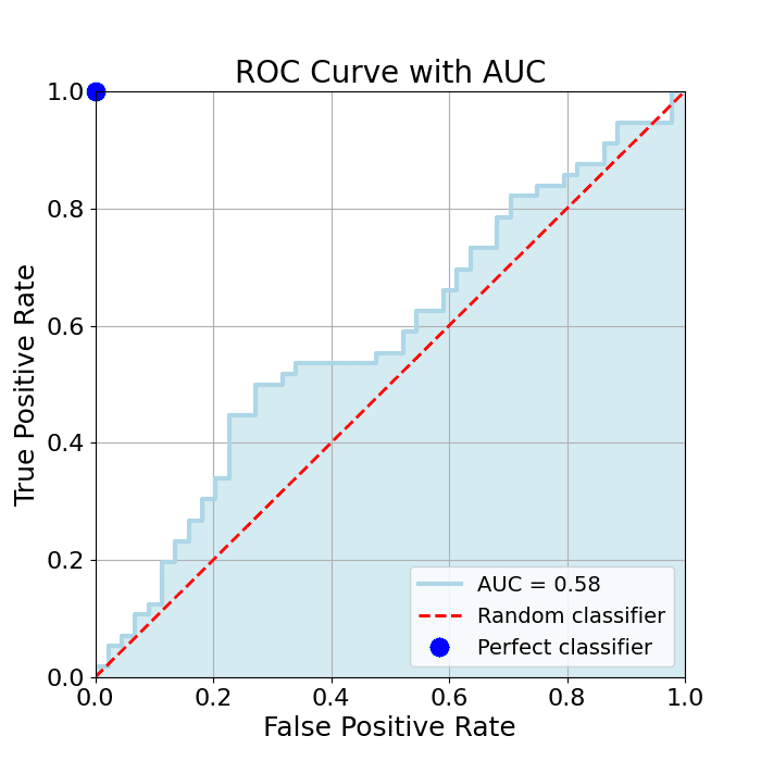
    AUC (Area Under the Curve) is a measure of a model’s ability to distinguish between positive and negative classes, based on the ROC (Receiver Operating Characteristic) curve. It quantifies the area under the ROC curve, where the curve represents the trade-off between the True Positive Rate (TPR) and False Positive Rate (FPR) at various thresholds.

    AUC Range:
    1.0: Perfect classifier
    0.5: Random guessing
    Below 0.5: Worse than random guessing, which rarely happens


    Login to view more content
  • ML0015 ROC Curve

    What is the ROC Curve, and how is it plotted?

    Answer

    The ROC (Receiver Operating Characteristic) curve is a graphical representation used to evaluate the performance of a binary classification model by comparing its True Positive Rate against its False Positive Rate at various threshold settings.

    Key Concepts:
    True Positive Rate (TPR): Also called sensitivity or recall, it measures the proportion of actual positives correctly identified.
    {\large \text{TPR} = \displaystyle\frac{\text{True Positives}}{\text{True Positives} + \text{False Negatives}}}
    False Positive Rate (FPR): The proportion of negatives incorrectly classified as positive.
    {\large \text{FPR} = \displaystyle\frac{\text{False Positives}}{\text{False Positives} + \text{True Negatives}}}
    Thresholds: Classification models output scores (often probabilities). A threshold determines the cutoff for labeling a prediction as positive or negative. The ROC curve is built by varying this threshold.

    Steps to Plot the ROC Curve:
    Train a Model: Train the binary classification model on the labelled dataset.
    Generate Probabilities: Instead of predicting class labels directly, generate probability scores for the positive class.
    Calculate TPR and FPR: Calculate the TPR and FPR for various threshold values
    Plot the Curve: Plot the TPR against the FPR for each threshold, creating the ROC curve.

    In an ROC curve:
    The x-axis shows FPR (1 – Specificity)
    The y-axis shows TPR (Sensitivity or Recall).
    Each point represents a TPR/FPR pair for a specific threshold.


    Login to view more content
  • ML0014 Confusion Matrix

    What is the confusion matrix?

    Answer

    A confusion matrix is a table that summarizes the performance of a classification model by comparing its predicted labels against the actual labels. For binary classification, it is typically organized into a 2×2 table containing:

    True Positives (TP): Cases where the model correctly predicts the positive class
    False Positives (FP): Cases where the model incorrectly predicts the positive class.
    False Negatives (FN): Cases where the model incorrectly predicts the negative class.
    True Negatives (TN): Cases where the model correctly predicts the negative class.

    It provides a detailed breakdown of the model’s predictions compared to the actual outcomes, which helps in understanding not only how many predictions were correct, but also the types of errors being made.


    Login to view more content

  • ML0013 Accuracy

    What is accuracy?

    Answer

    Accuracy in machine learning is a metric used to evaluate the performance of a model, particularly in classification tasks. It is the ratio of correct predictions to the total number of predictions made.
    Mathematically, it’s defined as:

    {\large \text{Accuracy} = \displaystyle\frac{\text{TP} + \text{TN}}{\text{TP} + \text{TN} + \text{FP} + \text{FN}}}

    If a model correctly predicts the class for 99 out of 100 samples, its accuracy is 99%.

    True Positives (TP): The model correctly predicts the positive class.
    False Positives (FP): The model incorrectly predicts the positive class (it predicted positive, but it was negative)
    True Negatives (TN): The model correctly predicts the negative class.
    False Negatives (FN): The model incorrectly predicts the negative class (it predicted negative, but it was positive).


    Login to view more content

  • ML0012 F1 Score

    What is F1 Score?

    Answer

    The F1 score is a crucial metric used to evaluate the performance of classification models, particularly when there’s an imbalance between the classes. It provides a balance between Precision and Recall, combining them into a single metric.

    {\large \text{F1 Score} = \displaystyle\frac{2 \times \text{Precision} \times \text{Recall}}{\text{Precision} + \text{Recall}}}


    Login to view more content
  • ML0011 Precision and Recall

    What are Precision and Recall?

    Answer

    Precision and recall are two fundamental metrics used to evaluate the performance of classification models, especially when dealing with imbalanced datasets or when the cost of different types of errors varies.

    Precision
    Precision (also known as positive predictive value) is the ratio of correctly predicted positive observations to the total predicted positives. In other words, it tells you, “When the model predicts a positive, how often is it right?” Mathematically, it’s defined as:

    {\large \text{Precision} = \displaystyle\frac{\text{True Positives (TP)}}{\text{True Positives (TP)} + \text{False Positives (FP)}}}

    For example, if a spam detector labels 100 emails as spam and 99 of them are actually spam, its precision is 99%.

    Recall
    Recall (also known as sensitivity or true positive rate) is the ratio of correctly predicted positive observations to all observations that are actually positive. It answers the question, “Out of all the actual positives, how many did the model capture?” Mathematically, it’s defined as:

    {\large \text{Recall} = \displaystyle\frac{\text{True Positives (TP)}}{\text{True Positives (TP)} + \text{False Negatives (FN)}}}

    For example, if there are 100 spam emails in total and the model correctly identifies 90 of them, its recall is 90%.

    True Positives (TP): The model correctly predicts the positive class.
    False Positives (FP): The model incorrectly predicts the positive class (it predicted positive, but it was actually negative)
    True Negatives (TN): The model correctly predicts the negative class.
    False Negatives (FN): The model incorrectly predicts the negative class (it predicted negative, but it was actually positive).


    Login to view more content
