Please compare max pooling and average pooling in deep learning, and explain in which scenarios you would prefer one over the other.
Answer
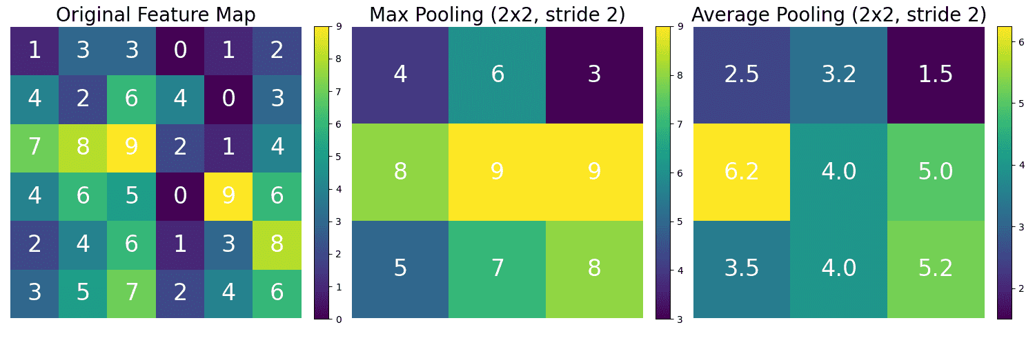
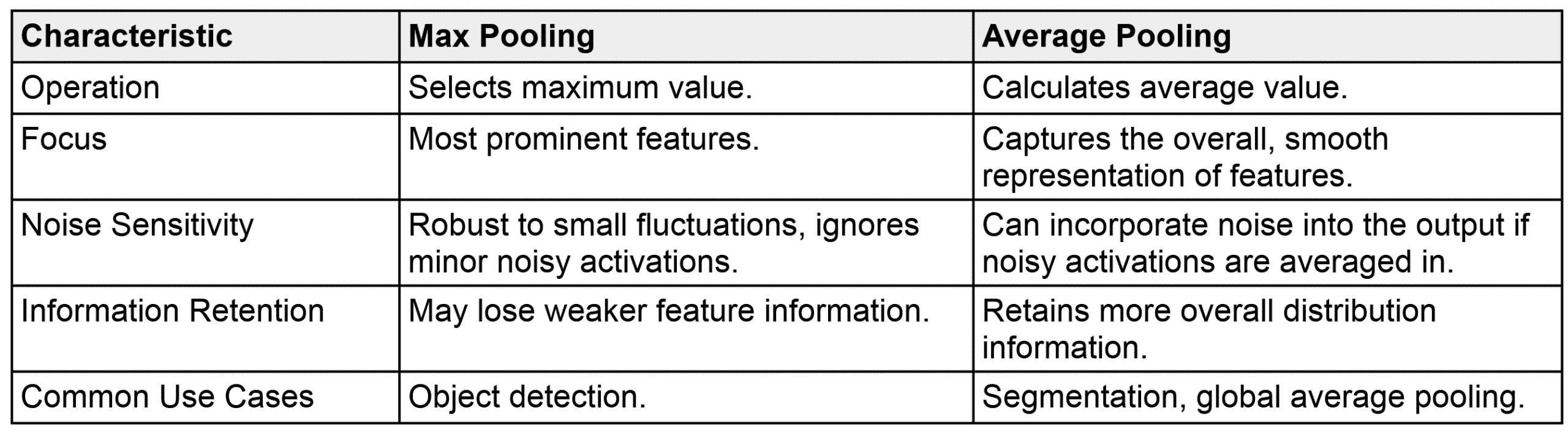
Max Pooling: Selects the maximum value within each non-overlapping window (kernel) of the feature map, downsampling while preserving the strongest activation in each region. Average Pooling: Computes the average of all values within each window of the feature map, downsampling by smoothing and retaining a holistic summary of the region.
The image below shows one example of Max Pooling and Average Pooling. Max Pooling VS Average Pooling in summary
What are the common strategies for Hyperparameter Tuning in deep learning?
Answer
Hyperparameter tuning in deep learning is the process of optimizing the configuration settings that control the learning process. (1) Manual/Heuristic Search: Start with values from prior work or common practice and iteratively adjust based on validation performance. (2) Grid Search: Exhaustively evaluates all combinations over a predefined, discrete grid of hyperparameter values; simple but scales poorly with dimensionality. (3) Random Search: Randomly sampling hyperparameter values from predefined ranges. (4) Bayesian Optimization: Using probabilistic models to intelligently suggest the next set of hyperparameters to try, balancing exploration and exploitation.
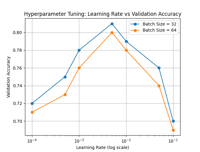
The below plot illustrates how validation accuracy varies with different learning rates (on a log scale) for two batch-size settings (32 and 64).
Why use batch normalization in deep learning training?
Answer
Batch normalization is a crucial technique during deep learning training that enhances network stability and accelerates learning. It achieves this by normalizing the inputs to the activation function for each mini-batch, specifically by subtracting the batch mean and dividing by the batch standard deviation.
After normalization, the layer applies a learnable scale (gamma) and shift (beta) that are updated during training to allow the network to recover the identity transformation if needed and to re-center/re-scale activations appropriately.
Here’s the formula for Batch Normalization: Where: represents an individual feature value in the batch. represents the mean of that feature across the current batch. represents the variance of that feature across the current batch. is a small constant (e.g. ) added to the denominator for numerical stability. is a learnable scaling parameter. is a learnable shifting parameter.
Batch Normalization is typically applied after the linear transformation of a layer (e.g., after the convolution operation in a convolutional layer) and before the non-linear activation function (e.g., ReLU).
The benefits of using Batch Normalization include: (1) Stabilizes learning: Reduces internal covariate shift, making training more stable and less sensitive to network initialization and hyperparameter choices. (2) Enables higher learning rates and accelerates training: Allows for larger learning rates without causing instability, leading to faster convergence. (3) Improves generalization: Normalizes each mini-batch independently, introducing noise into activations. This noise prevents over-reliance on specific mini-batch activations, forcing the network to learn more robust and generalizable features.
What are the common strategies for layer freezing in transfer learning?
Answer
Here are the common strategies for layer freezing in transfer learning: (1) Freeze all but the output layer(s): Train only the final classification/regression layers. Good starting point for similar tasks and small datasets. (2) Freeze early layers that capture general features: Train later, task-specific layers. Effective for moderately similar tasks. Balances leveraging pre-learned features with adapting higher-level representations. (3) Fine-tune all layers with a low learning rate: Adapt all weights slowly. Use with caution on small datasets. (4) Gradual Unfreezing: Start with frozen layers and progressively unfreeze layers during training to refine the model incrementally. Helps avoid large initial weight updates that can “destroy” learned features.
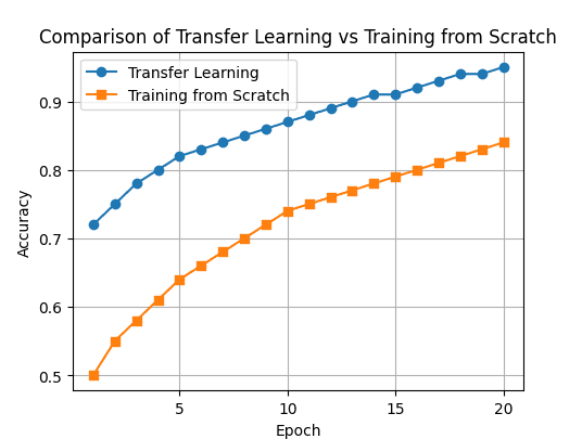
Why use transfer learning in deep learning instead of training from scratch?
Answer
Transfer learning can leverage knowledge from a pre-trained model to improve performance, reduce training time and data requirements, and lower computational costs when tackling a new but related task. (1) Leverages Existing Knowledge and Reduced Data Requirements: Transfer learning leverages learned useful representations from large datasets, which can achieve good performance with significantly less task-specific data. (2) Faster Convergence and Training Time: Starting with pre-trained weights provides a much better initialization point for training than random weights, leading to faster convergence and potentially better local optima. Pre-trained weights have already learned generalizable features, so fine-tuning on a new task typically requires much less training time. (3) Improved Performance on Limited Data Tasks: When data is limited, transfer learning often yields higher accuracy and better generalization compared to training a model from scratch.
What are the key advantages of using small convolutional kernels, such as 3×3, over utilizing a few larger kernels in deep learning architectures?
Answer
Using small convolutional kernels instead of a few larger kernels offers several significant advantages in deep learning architectures:
(1) Deeper Networks & More Non-Linearity: Stacking multiple 3×3 layers (e.g., three 3×3 layers) allows for a deeper network with more non-linear activation functions compared to a single large kernel. (2) Reduced Parameters: Multiple small kernels can achieve the same receptive field as a larger one, but with fewer parameters. Example: Two stacked 3×3 layers ( total parameters) have the same receptive field as a 5×5 layer ( total parameters) but fewer parameters. (3) Computational Efficiency: Fewer parameters in smaller kernels generally lead to lower computation costs during training and inference. (4) Gradual Receptive Field Expansion: Successive 3×3 convolutions progressively build a larger receptive field while maintaining fine detail. (3×3 filters focus on local detail capture with pixel neighborhoods, ideal for textures or edges.)
What are the benefits of using 1×1 convolutional layers in deep learning architectures?
Answer
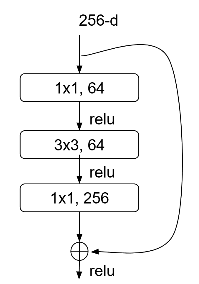
A 1×1 convolution, also known as a pointwise convolution, is a convolutional operation where the kernel size is 1×1, which plays several crucial roles in deep learning architectures. (1) Dimensionality control: 1×1 convolution can reduce or expand the number of feature maps, trading off representational capacity and computational cost.
For example, Bottleneck designs: In architectures like ResNet’s bottleneck block, a 1×1 conv first reduces channels (e.g., 256→64), then a 3×3 conv processes those, and finally another 1×1 conv expands back (64→256) to restore capacity while keeping compute manageable.
(2) Increased Network Depth with Controlled Cost: Allows for the design of deeper networks by reducing channel dimensionality before computationally expensive spatial convolutions. (3) Cross-Channel Feature Fusion: Enables interaction and combination of information across different feature channels at the same spatial location. (4) Non-linear mixing: When followed by activations (ReLU, etc.), 1×1 convolutions introduce non‐linear channel mixing that enhances model expressiveness.
What are the potential consequences of initializing all weights to one in a deep learning model?
Answer
Below are the key consequences of initializing all weights in a deep-learning model to one (a constant non-zero value), illustrating why random, scaled initializations (e.g., Xavier/He) are essential. (1) Symmetry Problem: Neurons receive identical gradients, causing them to learn the same features rather than developing distinct representations. (2) Limited Representational Capacity: The network cannot capture complex, varied patterns because all neurons behave identically. (3) Slow/No Convergence: The lack of Representational Capacity further makes it difficult for the model to update to the optimal weights. (The below image shows an example for training loss comparison for ones initialization vs random initialization) (4) Activation Saturation: Can push neurons into saturated regions of activation functions (e.g., sigmoid, tanh), leading to vanishing gradients.
Why are residual connections important in deep neural networks?
Answer
A residual connection (skip connection) adds a block input to a learned residual transformation, so the block learns an update rather than an entirely new mapping. For a shape-preserving block, the local Jacobian becomes , which supplies a direct identity component and creates shorter paths through the computational graph. This usually improves gradient propagation and optimization, but it does not guarantee nonzero or constant gradients: products of residual-block Jacobians can still shrink, grow, or cancel. Residual connections also address the degradation problem, in which adding layers to a plain network can increase training error because the deeper model is difficult to optimize even though an identity extension exists. These properties enabled effective training of ResNet architectures with hundreds of layers.
Figure 1: A shape-preserving block uses an identity shortcut, while a block that changes resolution or channel width uses a learned projection so the two paths have compatible shapes.
(1) Shorter Gradient Paths: An identity shortcut changes the local block Jacobian from to . The identity component gives backpropagation additional routes, although the product across many blocks can still vanish or explode.
(2) Identity Mapping Fallback: When an additional shape-preserving block is not useful, its residual branch can approach zero, making easier to represent than in a plain nonlinear stack.
(3) Easier Deep Optimization: Residual parameterization helps deeper models avoid the degradation problem, where added layers increase training error because optimization fails to recover a useful identity extension.
Mathematical Formulation:
Where:
is the input to residual block , and is its output.
is the learned residual branch parameterized by weights ; it learns an update to the shortcut representation.
is the residual-branch Jacobian, and is the identity operator with the same feature dimension as .
is an identity operator when input and output shapes match; otherwise it can be a learned projection, such as a strided convolution, that aligns spatial and channel dimensions.
Across residual blocks, backpropagation contains products of factors . These factors often improve conditioning relative to plain Jacobian products, but they do not impose a nonzero lower bound on gradient magnitude.
Figure 2: A plain stack multiplies full layer Jacobians, whereas a residual stack multiplies factors . The identity components provide additional gradient routes but do not guarantee stable magnitude.
What are the advantages and disadvantages of linear regression?
Answer
Linear regression aims to model the relationship between a dependent variable and one or more independent variables by fitting a linear equation to observed data.
Where represents the hypothesis (predicted value) for input feature vector x. is the bias (intercept) parameter, shifting the prediction up or down independent of features. are the weight parameters multiplying each feature. denotes the j‑th feature of the input vector x. is the total number of features (excluding the bias) used in the model.
Advantages: (1) Simplicity & Interpretability: Linear regression is easy to understand and implement. The coefficients of the model directly indicate the strength and direction of the relationship between the features and the target variable, making it highly interpretable. (2) Computational Efficiency: Its low computational cost makes linear regression fast to train, even on large datasets. (3) Effective for Linearly Separable Data: It performs well when the relationship between the independent and dependent variables is approximately linear.
Disadvantages: (1) Assumes Linearity: The primary limitation is the assumption that the relationship between the variables is linear. It will perform poorly if the underlying relationship is nonlinear. (2) Sensitivity to Outliers: Extreme values can disproportionately affect the model, distorting the results. (3) Multicollinearity Issues: When predictors are highly correlated, it becomes difficult to isolate individual effects, leading to unreliable coefficient estimates (4) Potential for Underfitting: The simplicity of the model may fail to capture the nuances and complexities of more intricate datasets.

 represents an individual feature value in the batch.
 represents the mean of that feature across the current batch.
 represents the variance of that feature across the current batch.
 is a small constant (e.g.
  ) added to the denominator for numerical stability.
  is a learnable scaling parameter.
 is a learnable shifting parameter.
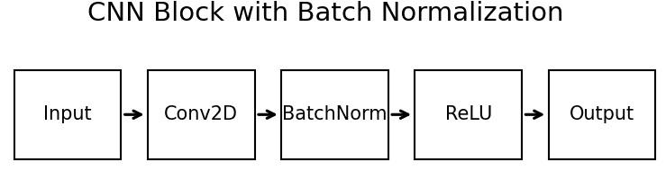
 total parameters) have the same receptive field as a 5×5 layer (
 total parameters) but fewer parameters.
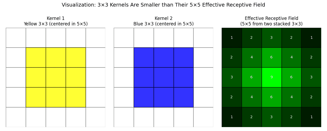

 , which supplies a direct identity component and creates shorter paths through the computational graph. This usually improves gradient propagation and optimization, but it does not guarantee nonzero or constant gradients: products of residual-block Jacobians can still shrink, grow, or cancel. Residual connections also address the degradation problem, in which adding layers to a plain network can increase training error because the deeper model is difficult to optimize even though an identity extension exists. These properties enabled effective training of ResNet architectures with hundreds of layers.
 so the two paths have compatible shapes.
 to
to  can approach zero, making
  easier to represent than in a plain nonlinear stack.


 is the input to residual block
  , and
, and  is its output.
 is the learned residual branch parameterized by weights
  ; it learns an update to the shortcut representation.
 is the residual-branch Jacobian, and
  is the identity operator with the same feature dimension as
  convolution, that aligns spatial and channel dimensions.
 residual blocks, backpropagation contains products of factors
  . These factors often improve conditioning relative to plain Jacobian products, but they do not impose a nonzero lower bound on gradient magnitude.

 represents the hypothesis (predicted value) for input feature vector x.
 is the bias (intercept) parameter, shifting the prediction up or down independent of features.
 are the weight parameters multiplying each feature.
 denotes the j‑th feature of the input vector x.
 is the total number of features (excluding the bias) used in the model.