Author: admin

  • ML0027 Leaky ReLU

    What are the benefits of the Leaky ReLU activation function?

    Answer

    Leaky ReLU modifies standard ReLU by replacing the hard zero on the negative side with a small linear slope: negative inputs pass through scaled by a small constant \alpha (typically 0.01). This one change directly attacks ReLU’s main weakness: the dying ReLU problem. Because the negative region now carries a small but non-zero gradient, a neuron whose pre-activation goes negative for all inputs still receives learning signal and can be pulled back into the active regime, instead of being frozen at zero output forever. At the same time Leaky ReLU retains everything that made ReLU attractive: the positive side stays the identity with gradient 1 (no vanishing gradients), the computation is still a trivial piecewise-linear threshold, and the output remains unbounded above, preserving ReLU’s scale behavior. In practice the accuracy gain over ReLU is often modest, but it costs nothing and removes a permanent failure mode.

    (1) Fixes Dying ReLU: Negative inputs get slope \alpha instead of 0, so gradient always flows and “dead” neurons can recover.
    (2) Keeps ReLU’s Strengths: Identity on the positive side (gradient 1, no saturation) and near-identical computational cost.
    (3) Costs: Introduces the hyperparameter \alpha (or learns it, as in PReLU); practical accuracy gains over ReLU are often small.

    ReLU versus Leaky ReLU curves with the small negative slope highlighted

    Figure 1: ReLU versus Leaky ReLU: identical on the positive side, but Leaky ReLU keeps a small slope \alpha in the negative region, enough gradient for a stuck neuron to recover instead of dying.

    Mathematical Formulation:
    \mathrm{LeakyReLU}(x) = x \text{ for } x \geq 0
    \mathrm{LeakyReLU}(x) = \alpha x \text{ otherwise}
    \alpha \approx 0.01
    \mathrm{LeakyReLU}'(x) = 1 \text{ for } x > 0
    \mathrm{LeakyReLU}'(x) = \alpha \text{ otherwise}

    Where:

    • x is the neuron’s pre-activation (weighted sum plus bias).
    • \alpha is the negative-side slope, a fixed small constant (0.01 by default) or a learned parameter in PReLU.
    FeatureReLULeaky ReLU
    Negative InputOutput is 0Output is a small non-zero value (αx)
    Gradient for x<00α (small positive constant)
    Dying ReLU ProblemSusceptibleLess susceptible
    Zero-Centered OutputNoNo (but closer than ReLU)
    Computational CostSlightly lowerSlightly higher

    Table 1: ReLU versus Leaky ReLU: the functions differ only in the negative region, but that small slope is what keeps neurons alive and gradients flowing.


    Login to view more content
  • ML0026 ReLU

    What are the benefits and limitations of the ReLU activation function?

    Answer

    ReLU (Rectified Linear Unit) is the piecewise-linear activation \max(0, x): it passes positive inputs unchanged and blocks negative ones to zero. Its benefits made it the default hidden-layer activation of deep learning: in the positive region the gradient is a constant 1, which largely eliminates the vanishing gradient problem that saturating sigmoid/tanh units suffer; negative outputs produce sparse activations, so only a subset of neurons is active at any time, yielding efficient and often more robust representations; and the function is a trivial threshold operation, far cheaper to compute than exponentials. Its main limitation is the dying ReLU problem: a neuron that falls into a regime of consistently negative pre-activations outputs zero and has zero gradient, so it can never recover, permanently shrinking model capacity. ReLU is also unbounded on the positive side (large activations can destabilize training if unmanaged) and non-differentiable at zero, a theoretical wrinkle handled in practice by defining a subgradient of 0 there.

    (1) Gradient Health: Derivative is 1 for x > 0: no saturation, strong gradient flow in deep networks.
    (2) Efficiency & Sparsity: A single comparison computes it; zero outputs give sparse, efficient representations.
    (3) Dying ReLU: Neurons stuck in the negative region output 0 with 0 gradient and may never recover; output is also unbounded above.

    ReLU curve passing positive inputs and zeroing negatives with the dead zone highlighted

    Figure 1: ReLU and its derivative: the identity ramp on the positive side keeps gradients at 1 (no vanishing), while the flat zero region on the left kills both signal and gradient, the source of the dying-ReLU failure mode.

    Mathematical Formulation:
    \mathrm{ReLU}(x) = \max(0, x)
    \mathrm{ReLU}'(x) = 1 \text{ for } x > 0, \quad 0 \text{ for } x \leq 0

    Where:

    • x is the neuron’s pre-activation (weighted sum plus bias).
    • \mathrm{ReLU}'(x) is the derivative used in backpropagation; at x = 0 the function is non-differentiable and implementations assign subgradient 0.

    Login to view more content
  • ML0025 Exploding Gradient

    What are the typical reasons for exploding gradient?

    Answer

    Exploding gradients occur when gradients grow exponentially during backpropagation, producing huge weight updates that make training unstable: the loss oscillates, spikes, or diverges to NaN. The mechanism mirrors the vanishing problem: the gradient at an early layer is a chain-rule product of per-layer factors, and when those factors are consistently larger than 1 in magnitude (from poorly scaled weight initialization, deep unnormalized architectures, or activation regimes with derivatives above 1), the product blows up with depth. Recurrent networks are especially vulnerable because the same weight matrix is multiplied once per time step, so long sequences amplify the effect. A learning rate set too high then converts already-large gradients into catastrophic updates.

    (1) Deep Chains of Large Factors: Products of weight matrices with spectral norm > 1 grow exponentially with depth (or RNN time steps).
    (2) Bad Initialization: Weights initialized too large produce outsized activations and derivatives from the start.
    (3) Compounding Learning Rate: A high learning rate turns large gradients into weight updates that overshoot and destabilize training.

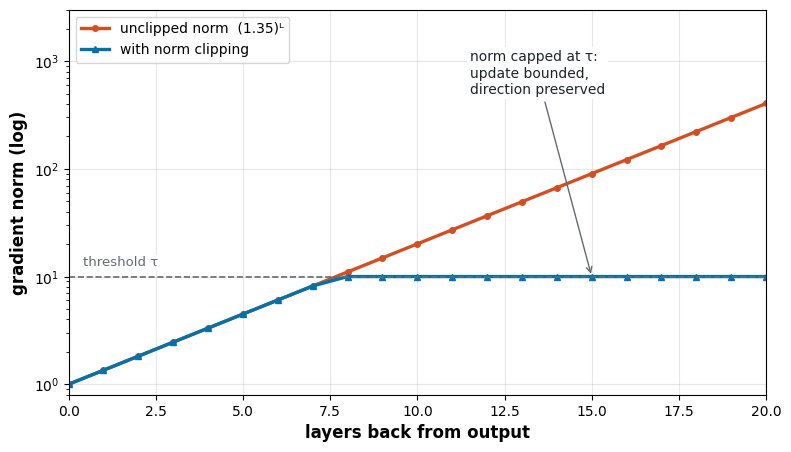
    Gradient norm exploding exponentially with depth and the same norm capped by gradient clipping

    Figure 1: Gradient norm flowing backward through a deep network: without control it grows geometrically layer by layer (note the log scale); gradient clipping caps the norm at a fixed threshold, keeping updates bounded regardless of depth.

    Mathematical Formulation:
    \frac{\partial L}{\partial z_l} = \frac{\partial L}{\partial z_n} \prod_{i=l}^{n-1} W_{i+1} \, f'(z_{i+1})
    \left\| \prod_i W_i \right\| \sim \prod_i \|W_i\|
    g \leftarrow g \cdot \min\!\left(1,\; \frac{\tau}{\|g\|}\right) \quad \text{(gradient clipping to threshold } \tau \text{)}

    Where:

    • z_l is the pre-activation of layer l; W_i and f'(z_i) are the per-layer weight and activation-derivative factors.
    • \|W_i\| is the operator (spectral) norm of the weight matrix; when the typical product exceeds 1, the gradient norm grows geometrically with depth.
    • g is the full gradient vector and \tau the clipping threshold: if \|g\| exceeds \tau, the gradient is rescaled down to norm \tau without changing its direction.

    Login to view more content
  • ML0024 Vanishing Gradient

    What are the typical reasons for vanishing gradient?

    Answer

    The vanishing gradient problem occurs when gradients shrink exponentially as they are backpropagated from the output layer toward the early layers of a deep network, so early layers receive almost no learning signal and train extremely slowly. The root cause is the chain rule: the gradient at an early layer is a product of many per-layer factors (weight matrices and activation derivatives), and if those factors are consistently smaller than 1 in magnitude, the product collapses toward zero as depth grows. The classic driver is saturating activation functions (sigmoid’s derivative peaks at only 0.25 and tanh’s at 1, and both are near zero for most of their input range), compounding with poor weight initialization that pushes pre-activations into the saturated tails. Recurrent networks suffer the same effect across time steps.

    (1) Saturating Activations: Sigmoid/tanh derivatives are small almost everywhere (sigmoid \sigma'(z) \leq 0.25); multiplying them across layers shrinks gradients exponentially.
    (2) Depth / Chain Rule: The gradient at layer 1 is a product of n per-layer factors; each factor below 1 makes the product vanish as n grows.
    (3) Poor Initialization: Too-large or too-small initial weights push activations into saturation, shrinking derivatives from the start.

    Gradient magnitude decaying exponentially with network depth on a log scale for sigmoid versus staying flat for ReLU

    Figure 1: Gradient magnitude at each layer during backpropagation (log scale): with sigmoid activations the signal decays roughly geometrically: after 20 layers the earliest layers receive gradients orders of magnitude smaller than the output layer.

    Mathematical Formulation:
    \frac{\partial L}{\partial z_l} = \frac{\partial L}{\partial z_{n}} \prod_{i=l}^{n-1} W_{i+1} \, f'(z_{i+1})
    \sigma(z) = \frac{1}{1 + e^{-z}}
    \sigma'(z) = \sigma(z)\big(1 - \sigma(z)\big) \leq 0.25

    Where:

    • z_l is the pre-activation of layer l, and n the total number of layers.
    • W_{i+1} is the weight matrix of layer i+1 and f'(\cdot) the activation derivative, the two per-layer factors in the chain product.
    • \sigma(z) is the sigmoid; its derivative peaks at 0.25 near z = 0 and approaches 0 in the saturated tails.
    Sigmoid curve with its derivative showing saturation regions where the derivative is near zero

    Figure 2: Why sigmoid kills gradients: outside the narrow active region around zero the derivative is essentially zero, so any neuron operating in the flat tails passes almost no gradient backward, and these small factors multiply down the chain.


    Login to view more content
  • ML0023 Gradient Descent

    What is Gradient Descent in machine learning?

    Answer

    Gradient descent is the iterative first-order optimization algorithm used to minimize a loss function by repeatedly stepping in the direction of steepest descent, opposite to the gradient. In each iteration the algorithm computes the gradient of the loss with respect to every parameter, then updates the parameters by subtracting a fraction of that gradient, where the fraction is the learning rate. The procedure repeats until the updates become negligibly small; for convex losses this converges to the global minimum, and for the non-convex losses of deep networks it reliably finds good local minima. In practice three variants trade gradient accuracy against computation: batch gradient descent uses the full dataset per step (stable but expensive), stochastic gradient descent uses a single sample (fast but noisy), and mini-batch gradient descent uses small subsets and is the default in modern training.

    (1) Update Rule: \theta \leftarrow \theta - \alpha \nabla_\theta J(\theta): move against the gradient, scaled by the learning rate.
    (2) Learning Rate: Too large diverges or oscillates; too small converges slowly; it is the single most important hyperparameter.
    (3) Variants: Batch (full data, stable), stochastic (one sample, noisy), mini-batch (compromise used in practice).

    Gradient descent steps converging down a one-dimensional parabola toward the minimum

    Figure 1: Gradient descent on a 1-D quadratic loss: each step moves opposite to the local slope, with step size proportional to the gradient: large steps far from the minimum, automatically shrinking steps near it.

    Mathematical Formulation:
    \theta_{t+1} = \theta_t - \alpha \, \nabla_\theta J(\theta_t)
    \nabla_\theta J(\theta) = \begin{bmatrix} \frac{\partial J}{\partial \theta_1} & \frac{\partial J}{\partial \theta_2} & \cdots & \frac{\partial J}{\partial \theta_p} \end{bmatrix}^{\top}

    Where:

    • \theta is the parameter vector being optimized (e.g., all network weights and biases).
    • \alpha is the learning rate, the step-size fraction applied to the gradient at each iteration.
    • J(\theta) is the loss (cost) function, and \nabla_\theta J its gradient: the vector of partial derivatives pointing in the direction of steepest ascent.

    Login to view more content
  • ML0022 Cross Entropy Loss

    Explain how Cross Entropy Loss is used for a classification task.

    Answer

    Cross-entropy loss (log loss) measures the distance between two probability distributions: the model’s predicted class probabilities and the true distribution (a one-hot vector for labeled data). Training a classifier means minimizing this distance, which is exactly maximum-likelihood estimation of the model parameters. In the binary case the loss averages -[y \log p + (1-y)\log(1-p)]; in the multi-class case only the true class term survives the one-hot sum, reducing the per-sample loss to -\log p_{\text{true}}. The logarithm is the key design choice: it penalizes confident wrong predictions severely: as the probability assigned to the true class approaches 0 the loss explodes toward infinity, giving a strong, well-behaved gradient exactly where the model errs most. It pairs naturally with sigmoid (binary) or softmax (multi-class) output layers, whose gradients under cross-entropy take the clean form p - y.

    (1) Definition: Negative log-likelihood of the true labels under the predicted distribution; minimizing it is maximum-likelihood training.
    (2) Confidence Sensitivity: Loss grows unboundedly as the true-class probability approaches 0; confident mistakes are punished hardest.
    (3) Standard Pairing: Sigmoid output + binary cross-entropy, softmax output + categorical cross-entropy; combined gradient simplifies to p - y.

    Cross entropy loss minus log p rising steeply as predicted probability of the true class approaches zero

    Figure 1: Per-sample loss -\log(p) as a function of the probability assigned to the true class: near p = 1 the loss is almost zero, below p = 0.1 it grows steeply: confident errors dominate the gradient.

    Mathematical Formulation:
    \mathcal{L}_{\text{binary}} = -\frac{1}{n} \sum_{i=1}^{n} \Big[ y_i \log p_i + (1 - y_i) \log(1 - p_i) \Big]
    \mathcal{L}_{\text{multi}} = -\frac{1}{n} \sum_{i=1}^{n} \sum_{c=1}^{C} y_{ic} \log p_{ic} = -\frac{1}{n} \sum_{i=1}^{n} \log p_{i,\text{true}}

    Where:

    • n is the number of samples and C the number of classes.
    • y_i \in \{0, 1\} is the true binary label; p_i the predicted probability of the positive class.
    • y_{ic} is the one-hot indicator (1 if sample i belongs to class c); p_{ic} the predicted probability of class c, so the inner sum keeps only the true-class term.

    Login to view more content
  • ML0021 L1 Loss L2 Loss

    What are the key differences between L1 loss and L2 loss?

    Answer

    L1 loss (mean absolute error) measures the average absolute difference between predictions and targets, while L2 loss (mean squared error) measures the average squared difference. That single change in the error function drives every practical difference: squaring amplifies large deviations, so L2 is more sensitive to outliers but enjoys a smooth gradient that shrinks to zero at the optimum; L1 treats all errors linearly, making it robust to outliers, but its gradient is a constant \pm 1 everywhere, so optimization can oscillate near the minimum instead of settling. When used as a regularization penalty rather than a regression loss, L1 additionally induces sparsity: it can drive the weights of uninformative features to exactly zero, performing implicit feature selection, whereas L2 only shrinks weights toward zero.

    (1) Error Measure: L1 averages absolute errors |e|; L2 averages squared errors e^2, amplifying large deviations.
    (2) Gradient Behavior: L1’s gradient is a constant \pm 1 (undefined at 0); L2’s gradient is proportional to the error and vanishes smoothly at the optimum.
    (3) Practical Choice: L1 for outlier-robust regression and sparse models; L2 for smooth, stable optimization when Gaussian noise is a reasonable assumption.

    FeatureL1 Loss (MAE)L2 Loss (MSE)
    Error CalculationAbsolute differenceSquared difference
    Outlier SensitivityLess sensitiveMore sensitive
    GradientConstant (+1 or -1)Proportional to the error
    SparsityInduces sparsity (feature selection)Does not inherently induce sparsity
    Optimization near minimumCan be unstableMore stable

    Table 1: The five practical differences between L1 and L2 loss; every row follows from the choice of |e| versus e^2 as the per-sample penalty.

    L1 absolute loss V-shape versus L2 squared loss parabola as functions of the residual

    Figure 1: Per-sample penalty as a function of the residual: L1 grows linearly (V-shape, robust to large errors), L2 grows quadratically (small errors are nearly free, large errors are heavily punished).

    Mathematical Formulation:
    \mathcal{L}_{L1} = \frac{1}{n} \sum_{i=1}^{n} \left| \hat{y}_i - y_i \right|
    \frac{\partial \mathcal{L}_{L1}}{\partial \hat{y}_i} = \frac{1}{n}\,\mathrm{sign}(\hat{y}_i - y_i)
    \mathcal{L}_{L2} = \frac{1}{n} \sum_{i=1}^{n} \left( \hat{y}_i - y_i \right)^2
    \frac{\partial \mathcal{L}_{L2}}{\partial \hat{y}_i} = \frac{2}{n}\left(\hat{y}_i - y_i\right)

    Where:

    • y_i is the true target and \hat{y}_i the model prediction for sample i.
    • n is the number of samples; both losses average over the dataset.
    • \mathrm{sign}(\cdot) is the sign function: +1 for positive residuals, -1 for negative, undefined at 0 (subgradient [-1, 1] in practice).
    Gradient of L1 loss constant step function versus gradient of L2 loss linear in the residual

    Figure 2: Gradient magnitude versus residual: L1’s constant gradient never decays (unstable near the optimum, undefined at zero), while L2’s gradient shrinks linearly and vanishes exactly at the optimum.


    Login to view more content
  • ML0020 Data Split

    How to split the dataset?

    Answer

    A dataset is typically split into three parts. The training set is used to fit the model: it learns the patterns and relationships from this data. The validation set is used during development to tune hyperparameters and compare model configurations, which prevents overfitting the training data. The test set is touched only once, for a final unbiased evaluation on completely unseen data: an estimate of real-world generalization. Typical ratios scale with dataset size: for small datasets (fewer than ~1,000 samples), 60–70% training / 10–15% validation / 15–25% test, with k-fold cross-validation strongly recommended because small validation estimates are noisy; for medium datasets (1,000–100,000), a common starting point is 70–80% / 10–15% / 10–15%; for large datasets (over ~100,000), even 98% / 1% / 1% leaves plenty of validation and test samples. For imbalanced data, use stratified splits so every part keeps the original class proportions.

    (1) Three Roles: Train fits, validation tunes, test judges; each set answers a different question.
    (2) Size-Dependent Ratios: Small data needs more training share plus cross-validation; big data can spare 1–2% for evaluation.
    (3) Stratification: Preserve class ratios in every split when classes are imbalanced.

    Train validation test split ratios for small, medium, and large datasets

    Figure 1: Split ratios by dataset size: the smaller the data, the larger the training share (and the more you need cross-validation); big data can evaluate on 1–2%.

    Mathematical Formulation:
    D = D_{\mathrm{train}} \cup D_{\mathrm{val}} \cup D_{\mathrm{test}}
    D_{\mathrm{train}} \cap D_{\mathrm{val}} = D_{\mathrm{train}} \cap D_{\mathrm{test}} = D_{\mathrm{val}} \cap D_{\mathrm{test}} = \emptyset

    Where:

    • D is the full dataset, partitioned into three disjoint subsets: no sample may appear in two roles.
    • D_{\mathrm{train}} is the training set used to fit the model parameters.
    • D_{\mathrm{val}} is the validation set used to tune hyperparameters and trigger early stopping.
    • D_{\mathrm{test}} is the test set, used exactly once for the final unbiased estimate; reusing it for tuning silently turns it into validation data.

    Login to view more content
  • ML0019 Imbalanced Data

    How to handle imbalanced data in Machine Learning?

    Answer

    Imbalanced data (where one class greatly outnumbers the other) skews models toward the majority class and must be handled deliberately. Five complementary techniques: resampling the dataset, by oversampling the minority class (e.g., SMOTE or ADASYN, which synthesize new minority points) or undersampling the majority class; data augmentation to create additional minority variants; class-weight adjustment, assigning a higher misclassification cost to the minority class during training; metric selection, evaluating with precision, recall, F1, or AUC-ROC rather than accuracy, which is misleading under imbalance; and algorithm selection, using specialized learners such as Balanced Random Forest or EasyEnsemble, or ensemble methods whose combined models are more robust to skewed classes.

    (1) Data-Level Fixes: Oversample the minority (SMOTE/ADASYN), undersample the majority, or augment minority samples.
    (2) Model-Level Fixes: Class weights in the loss, or imbalance-aware algorithms and ensembles.
    (3) Evaluation Fix: Never trust accuracy here; measure precision, recall, F1, or AUC.

    Imbalanced class distribution and SMOTE synthesizing minority samples

    Figure 1: Left: a 9:1 class imbalance. Right: SMOTE creates new minority points along the segments joining existing minority neighbors instead of duplicating them.

    Mathematical Formulation:
    x_{\mathrm{new}} = x_i + \lambda \, (x_{zi} - x_i), \quad \lambda \sim U(0,1)
    \mathcal{L} = \sum_{i} w_{y_i} \, \ell\big(f(x_i), y_i\big), \quad w_{c} \propto \frac{1}{n_c}

    Where:

    • x_{\mathrm{new}} is a synthetic minority sample created by SMOTE.
    • x_i is a minority sample and x_{zi} one of its nearest minority neighbors; \lambda is uniform in [0, 1], placing the new point somewhere on the connecting segment.
    • w_{y_i} is the per-sample weight from the class-weighting scheme; \ell is the per-sample loss and f the model.
    • n_c is the number of training samples of class c: the rarer the class, the higher its weight.

    Login to view more content
  • ML0018 Data Normalization

    Why is data normalization used in Machine Learning?

    Answer

    Data normalization scales features into a specific range or distribution: typically [0, 1] with min-max scaling, or mean 0 and standard deviation 1 with standardization, so that every feature contributes comparably to learning. It is used for three reasons. First, better model performance: algorithms built on distance metrics, such as k-nearest neighbors and SVMs, are skewed when one feature spans thousands and another spans decimals, normalization puts them on the same scale. Second, training stability and speed: normalized inputs keep neural network gradients well-conditioned, so training converges faster and more smoothly. Third, fair feature contribution: without scaling, large-magnitude features dominate the objective while small-magnitude ones are ignored, regardless of how informative they actually are.

    (1) What It Does: Rescales each feature to a common range (min-max) or distribution (z-score standardization).
    (2) Who Needs It: Distance-based models (kNN, SVM), gradient-based learners (neural networks, linear/logistic regression); tree ensembles largely do not.
    (3) The Payoff: Faster convergence, stabler training, and features competing on information rather than magnitude.

    Two-feature scatter before and after normalization

    Figure 1: Before: one axis spans hundreds while the other spans decimals, so distance is decided by the big axis alone. After standardization, both features contribute equally.

    Mathematical Formulation:
    x' = \frac{x - x_{\min}}{x_{\max} - x_{\min}}
    z = \frac{x - \mu}{\sigma}

    Where:

    • x' is the min-max normalized value of feature value x, squashed into [0, 1].
    • x_{\min} and x_{\max} are the feature’s minimum and maximum computed on the training set only.
    • z is the standardized (z-score) value with mean 0 and standard deviation 1.
    • \mu and \sigma are the feature’s training-set mean and standard deviation; fitting them on all data would leak test information.

    Login to view more content