Author: admin

ML0017 Data Augmentation
What are the common data augmentation techniques?
Answer
Data augmentation increases the diversity and effective size of a training set by creating modified versions of the existing data, especially valuable in computer vision and NLP, where collecting and labeling new data is expensive. In computer vision, common techniques are geometric transformations (rotate, flip, crop, scale), color adjustments (brightness, contrast, saturation, color jitter), and noise injection (random noise or blur). In NLP: synonym replacement, back translation (translate to another language and back), and random insertion or deletion of words. For tabular data: SMOTE-style synthetic sample generation and small random noise on numeric features. The benefits: better robustness and generalization, less overfitting (the model cannot memorize a moving target), relief for class imbalance, and lower data-collection cost.
(1) Core Idea: Apply label-preserving transformations so one sample teaches many variations of the same concept.
(2) By Data Type: Geometric/color/noise for images, synonym/back-translation/edit for text, SMOTE/noise for tables.
(3) Benefits: Robustness, regularization against overfitting, imbalance relief, and cost savings, all from data you already have.

Figure 1: One sample, five augmented views. The label never changes (only the appearance does), so the model learns invariance instead of memorizing pixels.
Mathematical Formulation:
$\tilde{x} = T(x; \phi), \quad \tilde{y} = y$
$\min_\theta \; \mathbb{E}_{(x,y)} \, \mathbb{E}_{\phi} \, \ell\big(f(T(x;\phi);\theta), y\big)$
Where:
$T(x;\phi)$ is the augmentation transform applied to sample $x$ with random parameters $\phi$ (e.g., rotation angle, crop offset).
$\tilde{x}$ is the augmented sample and $\tilde{y}$ its label, unchanged because the transforms are label-preserving.
$f(\cdot;\theta)$ is the model with parameters $\theta$ , and $\ell$ is the training loss.
$\mathbb{E}_{\phi}$ is the expectation over random augmentations: training minimizes loss over infinitely many variants, which is what regularizes the model.
Login to view more content
March 28, 2025
ML0016 AUC
What is AUC?
Answer
AUC (Area Under the Curve) measures a binary classifier’s ability to distinguish between the positive and negative classes, computed as the area under its ROC curve, the curve that trades off true positive rate against false positive rate across all thresholds. Its value ranges from 0 to 1: 1.0 is a perfect classifier, 0.5 is random guessing (the diagonal), and below 0.5 is worse than random, which rarely happens and can be flipped into a better model. AUC’s advantages: it is threshold-independent, summarizing performance over every decision threshold at once; it handles imbalanced data well because it evaluates the ranking of predictions rather than absolute counts; and it gives an intuitive single number for comparing different models.
(1) Definition: The area under the ROC curve: one scalar summarizing threshold-free discrimination.
(2) Probabilistic Meaning: AUC equals the probability that a random positive scores higher than a random negative.
(3) Reading The Scale: 1.0 perfect, 0.5 random, below 0.5 inverted.

Figure 1: AUC is literally the shaded area under the ROC curve; the wider the curve bows toward the top-left corner, the larger the area.
Mathematical Formulation:
$\text{AUC} = P\big(s(x^{+}) > s(x^{-})\big)$
$\text{AUC} = \int_{0}^{1} \text{TPR}(\text{FPR}) \, d\text{FPR}$
Where:
$s(x)$ is the model’s score (e.g., predicted probability) for sample $x$ .
$x^{+}$ is a randomly chosen positive sample and $x^{-}$ a randomly chosen negative one.
$\text{TPR}(\text{FPR})$ is the ROC curve itself, true positive rate as a function of false positive rate.
The two lines are equivalent: the geometric area (integral) equals the pairwise-ranking probability, which is why AUC measures ranking quality.
Login to view more content
March 27, 2025
ML0015 ROC Curve
What is the ROC Curve, and how is it plotted?
Answer
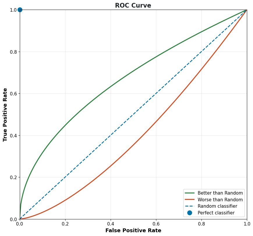
The ROC (Receiver Operating Characteristic) curve is a graphical tool for evaluating a binary classifier by plotting the true positive rate against the false positive rate at every classification threshold. Because models output scores rather than hard labels, a threshold decides what counts as positive; sweeping that threshold from strict to lenient traces out the curve. To plot it: train the binary classifier, generate probability scores for the positive class, compute TPR and FPR at many threshold values, then plot TPR versus FPR. Reading the curve: points near the top-left corner mean high TPR with low FPR: excellent performance; the diagonal is random guessing; curves below the diagonal are worse than random (and can be flipped to beat it); a perfect classifier sits at the single point (0, 1).
(1) Axes: Y is TPR (recall, sensitivity); X is FPR (1 − specificity); both sweep with the threshold.
(2) How It Is Built: Score the data, then recompute the confusion counts at every candidate threshold and connect the points.
(3) Reading It: Closer to the top-left corner is better; the diagonal is random; (0, 1) is perfect.

Figure 1: Reference ROC curves: the further a model bows toward the top-left corner, the better it ranks positives above negatives.
Mathematical Formulation:
$\text{TPR}(\tau) = \frac{TP(\tau)}{TP(\tau) + FN(\tau)}$
$\text{FPR}(\tau) = \frac{FP(\tau)}{FP(\tau) + TN(\tau)}$
Where:
$\tau$ is the classification threshold; varying it from 1 down to 0 traces the curve.
$TP(\tau)$ , $FP(\tau)$ , $FN(\tau)$ , and $TN(\tau)$ are the confusion-matrix counts at threshold $\tau$ .
$\text{TPR}$ is the true positive rate (same as recall) and $\text{FPR}$ is the false positive rate, the curve’s two axes.
Login to view more content
March 27, 2025

ML0014 Confusion Matrix

What is the confusion matrix?

Answer

A confusion matrix is a table that summarizes the performance of a classification model by comparing its predicted labels against the actual labels. For binary classification it is a 2×2 table with four cells: true positives (correctly predicted positive), false positives (negative predicted as positive), false negatives (positive predicted as negative), and true negatives (correctly predicted negative). Unlike a single scalar metric, it shows not only how many predictions were wrong but which kinds of errors were made. For multi-class problems, the matrix expands into a larger square table where cell $(i, j)$ counts the instances of actual class $i$ predicted as class $j$ ; off-diagonal clusters reveal which specific classes the model systematically confuses, guiding model refinement or relabeling.

(1) Structure: Rows are actual classes, columns are predicted classes; the diagonal holds all correct predictions.
(2) Binary Case: The four cells TP/FP/FN/TN feed every classification metric: accuracy, precision, recall, F1.
(3) Multi-Class Case: An $n \times n$ matrix whose off-diagonal hotspots expose systematic class confusions.

Actual \ Predicted	Predicted Positive	Predicted Negative
Actual Positive	True Positives (TP): correct positive	False Negatives (FN): missed positive
Actual Negative	False Positives (FP): false alarm	True Negatives (TN): correct negative

Mathematical Formulation:
$M_{ij} = \sum_{k=1}^{N} \mathbb{1}\big(y_k = i,\; \hat{y}_k = j\big)$
$\text{row-normalized:} \quad \tilde{M}_{ij} = \frac{M_{ij}}{\sum_j M_{ij}}$

Where:

$M_{ij}$ is the count in row $i$ , column $j$ of the confusion matrix.
$y_k$ is the true label of sample $k$ , $\hat{y}_k$ its predicted label, and $k\in\{1,\ldots,N\}$ indexes the $N$ samples.
$\mathbb{1}(\cdot)$ is the indicator function: 1 when the condition holds, 0 otherwise.
$\tilde{M}_{ij}$ is the row-normalized version: row $i$ then shows the per-class recall distribution, which reads better under class imbalance.

Three class confusion matrix heatmap with off-diagonal confusions

Figure 1: A 3-class example: strong diagonal means healthy classification; the bright off-diagonal cell shows the model systematically confuses class 1 with class 2.

March 22, 2025

ML0013 Accuracy
What is accuracy?
Answer
Accuracy is a metric that evaluates a classification model as the ratio of correct predictions to the total number of predictions: if a model classifies 99 of 100 samples correctly, its accuracy is 99%. It is intuitive and widely used because it directly answers “how often is the model right?” The four outcomes behind it are: true positives (positive correctly predicted), true negatives (negative correctly predicted), false positives (negative predicted as positive), and false negatives (positive predicted as negative). The important caveat: accuracy alone can be misleading on imbalanced data: a model that labels every patient “healthy” scores 99% on a dataset with 1% disease prevalence while being clinically useless. In such cases, precision, recall, and the F1 score give a truer picture.
(1) Definition: Correct predictions divided by all predictions, simple and intuitive.
(2) When It Works: Roughly balanced classes and symmetric error costs.
(3) The Accuracy Paradox: On skewed data, a trivial “always predict the majority” model scores high accuracy with zero real skill.

Figure 1: The accuracy paradox: with 90 negatives and 10 positives, predicting “negative” for everything yields 90% accuracy while catching zero positives.
Mathematical Formulation:
$\text{Accuracy} = \frac{TP + TN}{TP + TN + FP + FN}$
Where:
$TP$ and $TN$ are the counts of correct positive and negative predictions: the numerator counts everything the model got right.
$FP$ and $FN$ are the false alarm and miss counts; the denominator is simply the total number of samples.
Because $TN$ dominates on imbalanced data, high accuracy can hide a model that never identifies the minority class at all.
Login to view more content
March 22, 2025
ML0012 F1 Score
What is F1 Score?
Answer
The F1 score is a metric for classification models that combines precision and recall into a single number, and it is particularly useful when classes are imbalanced. It is the harmonic mean of the two: precision measures how many positive predictions are correct, recall measures how many actual positives are found, and the harmonic mean punishes imbalance between them: a high F1 requires both to be high at once. A model with 99% precision but 10% recall scores poorly on F1, because the harmonic mean is dominated by the smaller of the two values. This makes F1 a stricter, more informative summary than accuracy or either component alone when false positives and false negatives both matter.
(1) Definition: The harmonic mean of precision and recall, one number summarizing both.
(2) Key Property: It is dominated by the lower component, so it cannot be gamed by maximizing only precision or only recall.
(3) When To Use: Imbalanced classes, or when false positives and false negatives carry comparable cost.

Figure 1: F1 contour lines over the recall–precision plane: to reach a higher F1 band you must improve both metrics: moving along one axis alone quickly flattens out.
Mathematical Formulation:
$\text{F1} = \frac{2 \times \text{Precision} \times \text{Recall}}{\text{Precision} + \text{Recall}}$
$\text{F1} = \frac{2TP}{2TP + FP + FN}$
Where:
$\text{Precision}$ is $TP/(TP+FP)$ and $\text{Recall}$ is $TP/(TP+FN)$ (see the precision-and-recall question).
$TP$ , $FP$ , and $FN$ are the true positive, false positive, and false negative counts.
The second line is the equivalent counts-only form; $TN$ does not appear, which is why F1 stays meaningful under class imbalance.
Login to view more content
March 20, 2025
ML0011 Precision and Recall
What are Precision and Recall?
Answer
Precision and recall are two fundamental metrics for evaluating classification models, especially with imbalanced data or asymmetric error costs. Precision (positive predictive value) is the ratio of correctly predicted positives to all predicted positives: it answers “when the model says positive, how often is it right?” If a spam detector flags 100 emails and 99 are truly spam, precision is 99%. Recall (sensitivity, true positive rate) is the ratio of correctly predicted positives to all actual positives: it answers “of all the real positives, how many did the model catch?” If 100 spam emails exist and the model finds 90, recall is 90%. High precision means few false alarms (a spam filter that almost never marks good mail as spam); high recall means few misses (a cancer screening that almost never misses a real case). The two metrics sit on a trade-off controlled by the decision threshold.
(1) Precision = Accuracy Of Positive Predictions: Minimizing false positives matters when false alarms are costly.
(2) Recall = Coverage Of Actual Positives: Minimizing false negatives matters when misses are costly.
(3) Trade-Off: Lowering the classification threshold raises recall and usually lowers precision; raising it does the reverse.

Figure 1: The set view: precision is the share of the retrieved set that is correct, recall is the share of the relevant set that was retrieved.
Mathematical Formulation:
$\text{Precision} = \frac{TP}{TP + FP}$
$\text{Recall} = \frac{TP}{TP + FN}$
Where:
$TP$ (true positives) is the count of positives correctly predicted as positive.
$FP$ (false positives) is the count of negatives wrongly predicted as positive, the false alarms.
$FN$ (false negatives) is the count of positives wrongly predicted as negative, the misses.
$TN$ (true negatives) is the count of negatives correctly predicted as negative; it enters neither formula, which is why these metrics shine on imbalanced data.
Login to view more content
March 20, 2025
ML0010 Epoch Selection
What are effective strategies for selecting the appropriate number of training epochs in machine learning?
Answer
An epoch is one complete pass through the entire training dataset; choosing the right number of epochs means striking a balance between undertraining and overfitting. The effective strategies are: monitor validation metrics: if validation loss plateaus or starts increasing, further training adds nothing; implement early stopping: halt automatically when performance stops improving and keep the best weights; experiment: begin with a moderate range such as 10–100 epochs and adjust from the training/validation curves; and assess model and data complexity: complex models or datasets may need more epochs to capture the underlying patterns, while simpler problems converge quickly. Related definitions: an iteration is a single parameter update over one batch, so with 1,000 training samples and batch size 100, one epoch consists of 10 iterations.
(1) What An Epoch Is: One full pass over the training set; $N/B$ iterations per epoch for $N$ samples and batch size $B$ .
(2) Selection Strategy: Watch validation loss and let early stopping pick the epoch for you.
(3) Practical Range: Start around 10–100 epochs; scale up with task complexity, down for simple ones.

Figure 1: The validation curve answers “how many epochs”: stop in the sweet-spot zone: before it, the model is undertrained; after it, you are overfitting.
Mathematical Formulation:
$I = \frac{N}{B}$
$t^{*} = \arg\min_t \; \mathcal{L}_{\mathrm{val}}(t)$
Where:
$I$ is the number of iterations (parameter updates) in one epoch.
$N$ is the number of training samples and $B$ is the batch size.
$t^{*}$ is the ideal number of epochs, the one early stopping approximates.
$\mathcal{L}_{\mathrm{val}}(t)$ is the validation loss after $t$ epochs; its minimum marks the sweet spot in Figure 1.
Login to view more content
March 16, 2025
ML0009 Batch Size Selection
What are the best strategies for selecting the appropriate batch size?
Answer
Selecting an appropriate batch size is a crucial hyperparameter choice that trades training efficiency against optimization behavior. The practical strategy: start with a moderate value (16, 32, or 64) and adjust based on memory, gradient stability, and validation performance. Three factors drive the choice: memory constraints (larger batches need more GPU memory), dataset size (large datasets can sustain large batches; small datasets often benefit from the extra variability of small batches), and learning rate interaction (large batches usually allow (or require) a proportionally higher learning rate). Large batches train faster per epoch with stabler gradient estimates and higher memory cost, but can converge to sharp minima that generalize worse; small batches update more often with noisier gradients, which can explore flatter minima and generalize better at lower memory cost.
(1) Trade-Off Summary: Large batch = fast and stable but possibly sharp minima; small batch = slow and noisy but often better generalization.
(2) Practical Starting Points: Try 16/32/64 first, then scale with memory and dataset size.
(3) Interaction With LR: Scale the learning rate roughly proportionally when you change the batch size.

Figure 1: Same loss surface, two batch sizes: the small-batch path is noisy but wanders into a wider basin, while the large-batch path is smooth but direct.
Mathematical Formulation:
$\hat{g} = \frac{1}{B}\sum_{i=1}^{B}\nabla_\theta \mathcal{L}_i$
$\mathrm{Var}[\hat{g}] \propto \frac{\sigma^2}{B}$
Where:
$\hat{g}$ is the gradient estimate computed from one mini-batch.
$B$ is the batch size, and $i\in\{1,\ldots,B\}$ indexes the samples in the batch.
$\nabla_\theta \mathcal{L}_i$ is the per-sample loss gradient.
$\sigma^2$ is the per-sample gradient variance; doubling $B$ halves the gradient noise, which is why large batches give stable estimates and small batches give noisy ones.
Login to view more content
March 16, 2025
ML0008 Learning Rate Selection
What are the best practices for selecting an optimal learning rate?
Answer
Selecting an appropriate learning rate is one of the most important choices in training a neural network: it largely determines how quickly and how well the model learns. Four practices cover most situations. First, grid or random search over a range (e.g., 0.0001, 0.001, 0.01) while watching training performance, to narrow down an effective value. Second, use adaptive optimizers such as Adam, RMSProp, or Adagrad, which adjust the effective rate per parameter from gradient history and need less manual tuning. Third, apply learning rate schedules (step decay, exponential decay, or cosine annealing) that shrink the rate as training approaches convergence. Fourth, monitor the training loss: if it stops decreasing or oscillates, adjust the rate. Too high a rate overshoots the optimum and oscillates or diverges; too low a rate converges slowly or stalls; the right rate converges efficiently to a good solution.
(1) Why It Matters: The learning rate scales every update step; it is the single hyperparameter that most often decides whether training works at all.
(2) Four Practices: Search a range, prefer adaptive optimizers, decay the rate over time, and watch the loss curve.
(3) Diagnose From The Curve: Oscillating or rising loss means too high; an almost flat, slowly creeping loss means too low.

Figure 1: Reading the loss curve: too low creeps down slowly, a good rate drops fast and plateaus, too high oscillates and can diverge.
Mathematical Formulation:
$\theta_{t+1} = \theta_t - \eta_t \, \nabla_\theta \mathcal{L}(\theta_t)$
$\eta_t = \eta_0 \, \gamma^{\lfloor t / s \rfloor} \quad \text{(step decay)}$
Where:
$\theta_t$ denotes the model parameters at step $t$ .
$\eta_t$ is the learning rate at step $t$ , now time-dependent because of the schedule.
$\eta_0$ is the initial learning rate, $\gamma \in (0,1)$ is the decay factor, and $s$ is the number of steps between decays.
$\nabla_\theta \mathcal{L}(\theta_t)$ is the gradient of the training loss $\mathcal{L}$ , scaled by $\eta_t$ at every update.

Figure 2: Three standard schedules. All shrink $\eta_t$ over training so the model takes large steps early and fine steps near convergence.
Login to view more content
March 16, 2025