Category: Medium

  • DL0019 Go Deep

    How does increasing network depth impact the learning process?

    Answer

    Increasing network depth enhances feature learning and model capacity, but brings training instability, higher computational cost, and design complexity. Deeper stacks learn hierarchical representations (edges become textures, shapes, then objects) and can express certain complex functions far more efficiently than shallow networks, yet without modern techniques like residual connections and normalization, very deep networks are difficult or impossible to train.

    Benefits of Depth:

    (1) Improved Feature Hierarchy: Each layer composes the previous layer’s features, building increasingly abstract, high-level representations.
    (2) Increased Model Capacity: More layers let the network model more complex functions and patterns.
    (3) Exponential Efficiency for Complex Functions: Deep networks can represent some functions with vastly fewer units. For example, the n-input parity function needs roughly 2^{n-1} neurons in a single hidden layer but only about n small layers in a deep network.

    Challenges of Depth:

    (1) Vanishing/Exploding Gradients: Gradients shrink or grow multiplicatively through layers; without skip connections a 100-layer network may fail to train because gradients vanish before reaching early layers.
    (2) Increased Computational Cost: Deeper networks need significantly more compute and training time.
    (3) Higher Data Requirements: More parameters mean more overfitting risk unless the dataset grows correspondingly.

    Curve comparison showing a deep network tracking a complex high-frequency target function closely while a shallow network with a single hidden layer smooths over fine structure.

    Figure 1: A 6-layer network tracks the target’s high-frequency detail that a single-hidden-layer network smooths over. Depth buys compositional expressiveness.

    Where Depth Hurts Training: Each layer multiplies gradients by its Jacobian, so gradient magnitude behaves like a product of many factors; it collapses exponentially when those factors are consistently small.

    Log-scale chart of gradient norm per layer showing a plain deep network's gradients decaying exponentially into the vanishing zone while a residual network maintains healthy gradient magnitudes.

    Figure 2: In a plain deep network gradient norms decay exponentially toward the vanishing floor; skip connections keep gradients healthy across all 50 layers.

    Mathematical Formulation:
    \frac{\partial \mathcal{L}}{\partial x_1} = \prod_{l=1}^{L} J_l \cdot \nabla_{x_L}\mathcal{L}
    \lVert g_1 \rVert \approx \lVert \nabla_{x_L}\mathcal{L} \rVert \cdot \prod_{l=1}^{L} \sigma_l

    Where:

    • J_l is the Jacobian of layer l; gradients reaching the first layer are a product of L Jacobians.
    • \sigma_l is the dominant singular value of J_l; if most \sigma_l are below 1, the product, and hence \lVert g_1 \rVert, decays exponentially in L.
    • Residual blocks replace each factor with I + J_{F_l}, keeping the identity path alive so gradient norms stay near 1 even at 50+ layers.

    Login to view more content
  • DL0018 NaN Values

    What are the common causes for a deep learning model to output NaN values?

    Answer

    NaN outputs almost always trace back to numerical instability somewhere in the pipeline: unstable math operations, exploding gradients, an oversized learning rate, bad weight initialization, or corrupted input data. Once any parameter becomes NaN or Inf, the poisoning propagates through every subsequent layer, so the model’s outputs quickly become NaN everywhere.

    (1) Exploding Gradients: Gradients grow without bound through many layers, producing weight updates so large that parameters overflow to Inf/NaN.
    (2) Unstable Math Operations: \log(0), division by zero, or square roots of negative numbers yield Inf/NaN. For example, batch normalization divides by zero variance if a batch is constant and no \epsilon is used.
    (3) Improper Learning Rate: A learning rate that is too high makes parameter updates diverge, pushing weights to extreme values that overflow.
    (4) Incorrect Weight Initialization: Initializing weights to very large values can overflow activations on the very first forward pass.
    (5) Data Issues: Inputs containing NaN, Inf, or extreme unnormalized values inject invalid numbers directly into the computation graph.

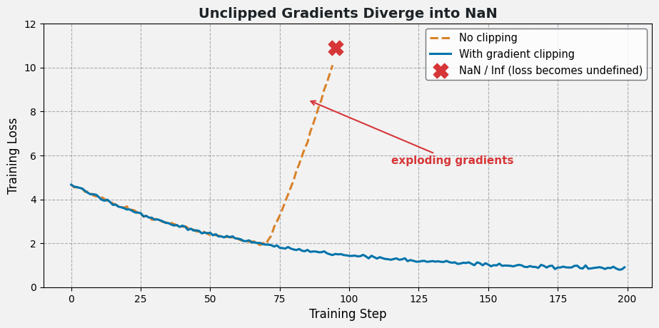
    Training loss curve where unclipped gradients explode and the loss becomes NaN, compared with stable training using gradient clipping.

    Figure 1: Unclipped gradients can explode within a few steps until the loss itself becomes NaN/Inf; gradient clipping keeps training on track.

    NaN Loss vs NaN Outputs: The two are stages of the same instability. A NaN loss can even appear while model outputs are still finite. For example, cross-entropy computes \log(\hat{y}), and a prediction extremely close to zero yields -\infty, which turns into NaN after the backward pass.

    Diagram of five common NaN causes with their standard fixes all feeding into NaN parameters and therefore NaN outputs.

    Figure 2: The five common causes and their standard fixes: every path ends at NaN parameters, hence NaN outputs.

    Mathematical Formulation:
    \mathcal{L} = -\log(\hat{y} + \epsilon)
    \hat{y} \to 0 \ \Rightarrow\ \mathcal{L} \to \infty \ \Rightarrow\ \text{NaN in backprop}
    g \leftarrow g \cdot \min\left(1,\ \frac{\tau}{\lVert g \rVert}\right)

    Where:

    • \hat{y} is the predicted probability of the true class; without the \epsilon clamp the loss diverges as \hat{y} approaches 0 and turns NaN in backprop.
    • g is the gradient vector and \tau the clipping threshold; the second rule (norm clipping) caps update magnitude before gradients can overflow the parameters.
    Login to view more content
  • DL0015 Cold Start

    What is a “cold start” problem in deep learning?

    Answer

    The cold start problem is the difficulty of making reliable predictions for new entities (users, items, or contexts) that have little or no historical data. Models that depend on past interactions, especially recommender systems built on collaborative filtering, have no signal to learn a meaningful representation of a brand-new user or item, so their predictions degrade to near-random or popularity-biased guesses until data accumulates.

    (1) Missing Interaction History: Collaborative filtering infers taste from a user-item matrix; a new row (user) or column (item) is empty, so the model cannot locate the entity in its embedding space.
    (2) Feedback Loop Risk: Poor early predictions reduce engagement, which further slows data collection for the new entity. The problem compounds itself.
    (3) Three Flavors: New-user cold start, new-item cold start, and new-system cold start (no data at all) each demand different remedies.

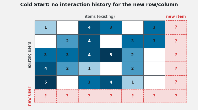
    User-item rating matrix with observed ratings shaded by value and a dashed red new-user row and new-item column filled with question marks to illustrate the cold start problem.

    Figure 1: The new user row and new item column contain no interactions. Collaborative filtering has nothing to condition on for them.

    Mitigation Strategies: The common theme is supplying side information until interaction data accumulates: transfer learning borrows representations from related domains; hybrid models mix collaborative signals with content features; and active onboarding explicitly gathers a few preferences from new users.

    (1) Transfer Learning / Pre-trained Models: Initialize from embeddings or models trained on similar tasks so the new domain starts from useful structure rather than random weights.
    (2) Hybrid Recommendation Models: Combine collaborative filtering with content-based features (user demographics, item metadata) so predictions remain reasonable with zero interactions.
    (3) Active Learning / User Onboarding: Ask new users to rate a handful of popular or diverse items, turning cold start into a short warm-up phase.

    Diagram of three mitigation strategies, transfer learning, hybrid model, and active onboarding, feeding into a recommender that produces reasonable predictions for new users and items.

    Figure 2: All three strategies inject auxiliary signal into the recommender so cold entities get reasonable predictions before their interaction rows fill in.

    Mathematical Formulation:
    \hat{r}_{ui} = \mu + b_u + b_i + p_u^{\top} q_i

    Where:

    • \hat{r}_{ui} is the predicted rating of user u for item i; \mu is the global mean rating.
    • p_u and q_i are the learned latent factor vectors for user u and item i; b_u, b_i are bias terms.
    • Cold start means p_u or q_i was never trained: with an empty interaction row/column, the factors stay at random init, so \hat{r}_{ui} is meaningless.

    Login to view more content
  • DL0014 Mixed Precision Training

    Can you explain the primary benefits of using mixed precision training in deep learning?

    Answer

    Mixed precision training runs the compute-heavy parts of a model in FP16 while keeping an FP32 master copy of the weights, so training gets the speed and memory of half precision without sacrificing final accuracy. Modern GPU/TPU tensor cores execute FP16 matrix math several times faster than FP32, and halving activation memory lets you train larger models or use larger batches on the same hardware.

    (1) Faster Training: FP16 tensor-core matmuls deliver up to an order of magnitude more throughput than FP32 on supported hardware (e.g., ~312 vs ~19.5 TFLOPS on an A100).
    (2) Reduced Memory Usage: FP16 activations and working weight copies occupy half the bytes, freeing room for larger batch sizes or deeper models (master weights and optimizer states stay FP32, so total training memory falls by less than half).
    (3) Maintained Accuracy: FP32 master weights plus loss scaling keep small gradient values representable, so final model quality matches full-precision training.

    Bit layout comparison of FP32 with 8 exponent and 23 mantissa bits versus FP16 with 5 exponent and 10 mantissa bits, showing the reduced dynamic range of FP16.

    Figure 1: FP16 trades exponent range and mantissa precision for half the storage: gradients below 6.1 \times 10^{-5} would underflow to zero without loss scaling.

    The Training Loop: Weights are stored in FP32 as the master copy. Each step casts them to FP16 for the forward and backward passes, multiplies the loss by a scale factor S so that FP16 gradients stay in range, then divides the gradients by S and applies the optimizer update to the FP32 master weights.

    Mixed precision training loop diagram showing FP32 master weights cast to FP16 for forward and backward passes with loss scaling, then unscaled gradients updating the FP32 master copy.

    Figure 2: FP16 does the heavy math while the FP32 master copy absorbs tiny updates; loss scaling S shifts gradients into FP16’s representable range.

    Measured Benefits: On tensor-core hardware the speedup is substantial, and the halved activation memory (the dominant term at large batch sizes) directly translates into larger feasible models or batches.

    Bar charts comparing FP32 versus mixed precision on tensor-core throughput and per-parameter memory footprint.

    Figure 3: Roughly 16x tensor-core throughput and half the activation memory are the headline wins; with Adam states kept in FP32, per-parameter training memory drops only modestly.

    Mathematical Formulation:
    \mathcal{L}' = S \cdot \mathcal{L}
    g_{fp32} = \frac{1}{S}\,\nabla_{\theta}\mathcal{L}'
    \theta \leftarrow \theta - \eta\, g_{fp32}

    Where:

    • S is the loss-scale factor (e.g., 2^{15}, or dynamically adjusted); \mathcal{L}' is the scaled loss used for backprop in FP16.
    • \nabla_{\theta}\mathcal{L}' are the scaled FP16 gradients; dividing by S restores the true gradient g_{fp32}.
    • \theta is the FP32 master weight set and \eta the learning rate; updates always land on the master copy.

    Costs to Manage: FP16’s narrow range causes gradient underflow and occasional activation overflow, requiring loss scaling and careful debugging of NaN/Inf values; efficiency also depends on hardware with fast FP16 paths.


    Login to view more content
  • DL0013 Instance Normalization

    Can you explain what Instance Normalization is in the context of deep learning?

    Answer

    Instance Normalization (IN) normalizes each individual sample and each channel independently: for every (instance, channel) pair it subtracts the mean and divides by the standard deviation computed over that feature map’s spatial dimensions only. Because statistics never cross instance boundaries, IN is unaffected by mini-batch composition and works with batch size 1. This per-instance normalization removes sample-specific contrast and style, which is why IN became the standard in style transfer and image-generation models.

    (1) Per-Instance, Per-Channel Statistics: Mean and variance are computed over the H \times W spatial positions of each channel of each sample separately, so no information leaks across the batch.
    (2) Batch-Size Independent: Statistics do not depend on other samples, so IN behaves identically at training and test time and remains stable with small batches.
    (3) Removes Instance-Specific Style: Normalizing each map’s contrast discards style-like appearance information while preserving content structure, which suits style transfer, GANs, and domain adaptation.

    Side-by-side diagram of batch normalization sharing per-channel statistics across all instances versus instance normalization computing statistics within each instance-channel feature map.

    Figure 1: BN pools statistics per channel across the whole batch (red dashed groups), while IN normalizes each (instance, channel) map alone (orange dashed boxes): the source of IN’s batch independence.

    Mathematical Formulation:
    \mu_{nc} = \frac{1}{HW} \sum_{h=1}^{H} \sum_{w=1}^{W} x_{nchw}
    \sigma_{nc}^2 = \frac{1}{HW} \sum_{h=1}^{H} \sum_{w=1}^{W} (x_{nchw} - \mu_{nc})^2
    \hat{x}_{nchw} = \frac{x_{nchw} - \mu_{nc}}{\sqrt{\sigma_{nc}^2 + \epsilon}}
    y_{nchw} = \gamma_c\,\hat{x}_{nchw} + \beta_c

    Where:

    • x_{nchw} is the input activation at batch index n, channel c, spatial position (h, w).
    • \mu_{nc} and \sigma_{nc}^2 are the mean and variance over the H \times W spatial extent of instance n, channel c.
    • \hat{x}_{nchw} is the normalized activation; \epsilon is a small constant for numerical stability.
    • \gamma_c and \beta_c are learnable per-channel scale and shift parameters; y_{nchw} is the output.

    Contrast with Batch Normalization: BN computes per-channel statistics over the entire mini-batch (N \times H \times W), which couples a sample’s output to its batchmates and forces a switch to running averages at inference. IN’s per-sample statistics are identical in both phases, and discarding per-instance contrast is precisely what removes style from content images.

    FeatureInstance Normalization (IN)Batch Normalization (BN)
    Scope of statsPer instance, per channel (over H \times W)Per channel (over N \times H \times W)
    Batch sizeIndependent; works with batch = 1Dependent; needs stable batch stats
    Primary useStyle transfer, GANs, domain adaptationImage classification, general CNNs
    EffectRemoves instance-specific style/contrastStabilizes training, speeds convergence
    InferenceSame per-sample stats at test timeUses running stats from training

    Bottom line: IN removes per-instance contrast (style); BN aligns feature scales across the batch. IN trades BN’s cross-sample regularization for batch independence and style removal.


    Login to view more content
  • DL0012 Zero Padding

    Why is zero padding used in deep learning?

    Answer

    Zero padding adds rows and columns of zeros around the input before a convolution. In CNNs it preserves spatial dimensions, prevents border information from being under-sampled, allows larger kernels and deeper stacks, and gives explicit control over output size. Beyond CNNs, padding standardizes variable-length sequences so NLP and time-series models can process them in batches.

    (1) Preserves Spatial Dimensions: Without padding (“valid” convolution), a k \times k kernel shrinks the feature map by k - 1 in total per dimension ((k-1)/2 per side) each layer; padding with p = (k-1)/2 keeps the size unchanged.
    (2) Retains Boundary Information: Padded borders let the kernel center on edge pixels, so corners and boundaries are processed as thoroughly as the interior.
    (3) Controls Output Size: Padding decouples output dimensions from kernel size, enabling deeper networks and predictable feature-map shapes.

    Mathematical Formulation:
    n_{out} = \left\lfloor \frac{n_{in} + 2p - k}{s} \right\rfloor + 1

    Where:

    • n_{out} and n_{in} are the output and input spatial sizes.
    • p is the padding width added to each side, k is the kernel size, and s is the stride.
    • “Same” padding for stride 1 uses p = (k-1)/2, giving n_{out} = n_{in}.
    2D convolution example showing a 4x4 input padded with one ring of zeros into 6x6, so a 3x3 kernel produces a same-size 4x4 output.

    Figure 1: Padding a 4 \times 4 input to 6 \times 6 lets a 3 \times 3 kernel output the same 4 \times 4 size instead of shrinking to 2 \times 2.

    Beyond CNNs: In NLP and time-series tasks, zero padding extends shorter sequences to a uniform length for efficient batching. Because padded positions carry no information, models combine padding with attention masks so Transformer self-attention ignores those positions entirely.

    Three panels comparing valid convolution without padding, same convolution with padding, and NLP sequence padding with an attention mask.

    Figure 2: Valid shrinks the map, same preserves it, and sequence padding plus a mask enables batched NLP inputs.


    Login to view more content
  • DL0010 Receptive Field

    What is the receptive field in convolutional neural networks, and how do you calculate it?

    Answer

    The receptive field (RF) of a neuron is the region of the input image that can influence that neuron’s activation. It grows with network depth, so deeper layers see larger context and learn more hierarchical features. The RF is computed layer by layer: each layer expands the field according to its kernel size, scaled by the cumulative stride of all preceding layers.

    (1) Definition: The RF is the input region that affects one activation in a given layer; a neuron with a large RF integrates global context.
    (2) Growth Rule: Each layer adds (k_l - 1) \times \prod s_i to the RF, where k_l is the kernel size and the product runs over all previous strides.
    (3) Design Implication: Stacked small kernels grow the RF parameter-efficiently; strided and dilated convolutions grow it much faster.

    Mathematical Formulation:
    RF_l = RF_{l-1} + (k_l - 1) \times \prod_{i=1}^{l-1} s_i

    Where:

    • RF_l is the receptive field size after layer l, with RF_0 = 1 at the input layer.
    • k_l is the kernel size of layer l.
    • s_i is the stride of layer i, and the product accumulates all strides before layer l.
    Stacked feature map rows showing the receptive field of one neuron growing from 3 to 5 to 7 input cells across three 3x3 convolution layers with stride 1.

    Figure 1: With k=3, s=1 per layer, one neuron’s RF grows from 3 to 5 to 7 input cells as layers stack.

    Stride and Dilation Effects: A layer with stride 2 doubles the jump between adjacent neurons, so every subsequent layer adds twice as much to the RF. Dilated convolutions enlarge the kernel’s span by inserting gaps, growing the RF without reducing resolution, which is useful in segmentation.

    Worked receptive field calculation across four layers showing RF values 1, 3, 5, 7, 11 with the contribution of a stride-2 layer multiplying later increments.

    Figure 2: Worked example: a stride-2 layer at l=3 doubles the increment contributed by every later layer, jumping the RF from 7 to 11.

    Real CNN Stacks: In practice, convolutions, pooling, and dilation mix freely: pooling multiplies the jump between neurons, and dilated kernels widen the span, so the RF can reach 22 within just five layers.

    Line chart of receptive field size growing from 1 to 22 across a CNN stack with convolutions, max pooling, and a dilated convolution.

    Figure 3: In a realistic stack, max pooling doubles the jump and dilation (D=2) widens the kernel, pushing the RF from 1 to 22 in five layers.


    Login to view more content
  • DL0003 1×1 Convolution

    What are the benefits of using 1×1 convolutional layers in deep learning architectures?

    Answer

    A 1×1 convolution (pointwise convolution) operates on the channel dimension at each spatial location, enabling dimensionality control, cross-channel feature fusion, and non-linear mixing, all with minimal computational cost. In architectures like ResNet’s bottleneck block, a 1×1 conv first reduces channels (e.g., 256→64), a 3×3 conv processes the reduced representation, and another 1×1 conv expands back (64→256), restoring capacity while keeping compute manageable. This design allows deeper networks without prohibitive parameter growth.

    (1) Dimensionality Control: 1×1 convolutions can reduce or expand the number of feature maps, trading off representational capacity and computational cost as needed.
    (2) Depth With Controlled Cost: By reducing channel dimensionality before expensive spatial convolutions, 1×1 convs enable deeper architectures without the quadratic growth in channel count that a plain 3 \times 3 block incurs.
    (3) Cross-Channel Feature Fusion: Each output pixel is a learned linear combination of all input channels at that location, enabling rich channel-wise interactions.
    (4) Non-Linear Mixing: When followed by activations (ReLU, etc.), 1×1 convs introduce non-linear channel mixing that enhances model expressiveness.

    1x1 convolution operation showing per-pixel cross-channel weighted sum across input channels to produce one output channel.

    Figure 1: A 1×1 convolution performs a per-pixel weighted sum across all input channels: each output channel is a learned linear combination of every input channel at the same spatial position, preserving H\times W.

    Mathematical Formulation:
    y_{i,j,c_{out}} = \sum_{c_{in}=1}^{C_{in}} w_{c_{in},c_{out}} \cdot x_{i,j,c_{in}} + b_{c_{out}}
    \text{FLOPs}_{1\times1} = H \times W \times C_{in} \times C_{out}

    Where:

    • x_{i,j,c_{in}} is the input activation at spatial position (i,j) in channel c_{in}; y_{i,j,c_{out}} is the output.
    • w_{c_{in},c_{out}} is the 1×1 kernel weight connecting input channel c_{in} to output channel c_{out}; there is no spatial kernel dimension.
    • C_{in} and C_{out} are the input and output channel counts; b_{c_{out}} is the bias for each output channel.
    • H and W are the spatial height and width of the feature map; the operation is equivalent to a fully-connected layer applied per-pixel across channels.
    ResNet bottleneck block showing 1x1 convolutions reducing then expanding channels around a 3x3 convolution.

    Figure 2: ResNet bottleneck block: a 1×1 conv reduces channels (256→64), a 3×3 conv processes the compressed representation, and another 1×1 conv expands back (64→256), with a residual skip connection.


    Login to view more content
  • DL0002 All Ones Init

    What are the potential consequences of initializing all weights to one in a deep learning model?

    Answer

    Initializing all weights to one (or any constant non-zero value) creates a symmetry problem: every neuron in the same layer receives identical gradients, so they learn the same features and cannot develop diverse representations. This limits the network to a single effective feature per layer, severely reducing its representational capacity. Training becomes slow or fails to converge because the optimizer cannot differentiate between neurons. Additionally, constant positive weights can push activations into saturated regions of sigmoid or tanh, worsening vanishing gradients.

    (1) Symmetry Problem: All neurons in a layer receive the same input and the same gradient, so they evolve identically throughout training.
    (2) Limited Representational Capacity: The network behaves as if each layer has only one neuron, making it impossible to capture complex, varied patterns in the data.
    (3) Slow or Failed Convergence: Because neurons cannot differentiate, the loss landscape lacks the diversity needed for gradient descent to find useful minima.
    (4) Activation Saturation: Uniform positive weights shift pre-activation values into the flat tails of sigmoid and tanh, producing vanishing gradients that stall learning.

    Symmetry problem visualization comparing all-ones initialization where neurons collapse versus random initialization with diverse features.

    Figure 1: The symmetry problem: with all-ones weights every neuron computes the same function and receives the same gradient, while random initialization lets each neuron learn a distinct feature.

    Mathematical Formulation:
    \frac{\partial \mathcal{L}}{\partial w_{ij}^{(l)}} = \delta_i^{(l)} \cdot a_j^{(l-1)}
    w_{ij}^{(l)} = 1 \quad \forall\, i,j \implies \delta_i^{(l)} = \delta_j^{(l)} \quad \forall\, i,j

    Where:

    • w_{ij}^{(l)} is the weight from neuron j in layer l-1 to neuron i in layer l.
    • \delta_i^{(l)} is the error signal (delta) for neuron i in layer l.
    • a_j^{(l-1)} is the activation of neuron j in the previous layer.
    • \mathcal{L} is the loss function; when all weights are equal, all delta signals are identical, so every weight updates by the same amount.
    Training loss comparison between ones initialization and random initialization showing slow convergence for constant weights.

    Figure 2: Training loss comparison: ones initialization converges slowly and plateaus at a high loss, while random initialization descends rapidly to a low minimum.


    Login to view more content
  • DL0001 Residual Connection

    Why are residual connections important in deep neural networks?

    Answer

    A residual connection (skip connection) adds a block input to a learned residual transformation, so the block learns an update rather than an entirely new mapping. For a shape-preserving block, the local Jacobian becomes I+J_F, which supplies a direct identity component and creates shorter paths through the computational graph. This usually improves gradient propagation and optimization, but it does not guarantee nonzero or constant gradients: products of residual-block Jacobians can still shrink, grow, or cancel. Residual connections also address the degradation problem, in which adding layers to a plain network can increase training error because the deeper model is difficult to optimize even though an identity extension exists. These properties enabled effective training of ResNet architectures with hundreds of layers.

    (1) Shorter Gradient Paths: An identity shortcut changes the local block Jacobian from J_F to I+J_F. The identity component gives backpropagation additional routes, although the product across many blocks can still vanish or explode.
    (2) Identity Mapping Fallback: When an additional shape-preserving block is not useful, its residual branch F_l(x_l) can approach zero, making x_{l+1}\approx x_l easier to represent than in a plain nonlinear stack.
    (3) Easier Deep Optimization: Residual parameterization helps deeper models avoid the degradation problem, where added layers increase training error because optimization fails to recover a useful identity extension.

    Comparison of shape-preserving residual blocks with identity shortcuts and shape-changing blocks with learned projection shortcuts.

    Figure 1: A shape-preserving block uses an identity shortcut, while a block that changes resolution or channel width uses a learned projection S_l so the two paths have compatible shapes.

    Mathematical Formulation:
    x_{l+1}=F_l(x_l;W_l)+x_l
    \frac{\partial x_{l+1}}{\partial x_l}=J_{F_l}+I
    x_{l+1}=F_l(x_l;W_l)+S_lx_l

    Where:

    • x_l is the input to residual block l, and x_{l+1} is its output.
    • F_l(x_l;W_l) is the learned residual branch parameterized by weights W_l; it learns an update to the shortcut representation.
    • J_{F_l}=\partial F_l/\partial x_l is the residual-branch Jacobian, and I is the identity operator with the same feature dimension as x_l.
    • S_l is an identity operator when input and output shapes match; otherwise it can be a learned projection, such as a strided 1\times1 convolution, that aligns spatial and channel dimensions.
    • Across L residual blocks, backpropagation contains products of factors I+J_{F_l}. These factors often improve conditioning relative to plain Jacobian products, but they do not impose a nonzero lower bound on gradient magnitude.
    Backward-path comparison showing full Jacobian products in plain stacks and identity-plus-residual Jacobian products in residual stacks.

    Figure 2: A plain stack multiplies full layer Jacobians, whereas a residual stack multiplies factors I+J_{F_l}. The identity components provide additional gradient routes but do not guarantee stable magnitude.


    Login to view more content