Interview for Machine Learning

Category: Medium

DL0037 Transformer Architecture III
Why do Transformers use a dot product, rather than addition, to compute attention scores?
Answer
Dot product attention is a fast and naturally aligned similarity measure; with scaling, it remains numerically stable and highly parallelizable, which is why Transformers prefer it over addition.
(1) Dot product captures similarity: The dot product between query $q$ and key $k$ grows larger when they point in similar directions, making it a natural similarity measure.
The scores are normalized with Softmax and have probabilistic interpretations:
$\alpha_i = \frac{e^{q \cdot k_i}}{\sum_{j=1}^K e^{q \cdot k_j}}$
Where:
$q \cdot k_i$ is the dot product similarity between query and key.
The figure below illustrates the dot product for measuring similarity.

(2) Efficient computation: Dot products can be computed in parallel as a matrix multiplication $QK^\top$ , which is hardware-friendly.
Login to view more content
August 26, 2025
DL0029 Dilated Attention
Could you explain the concept of dilated attention in transformer architectures?
Answer
Dilated attention introduces gaps between attention positions to sparsify computation, enabling efficient long-range dependency modeling. It is particularly helpful in tasks requiring scalable attention over long sequences. It trades off some granularity for global context by spreading attention more widely and sparsely.
Dilated attention is similar to dilated convolutions in CNNs, where gaps (dilations) are introduced between the sampled positions.
Instead of attending to all tokens (as in standard self-attention), each query token attends to every d-th token. This dilation rate controls the stride in attention.
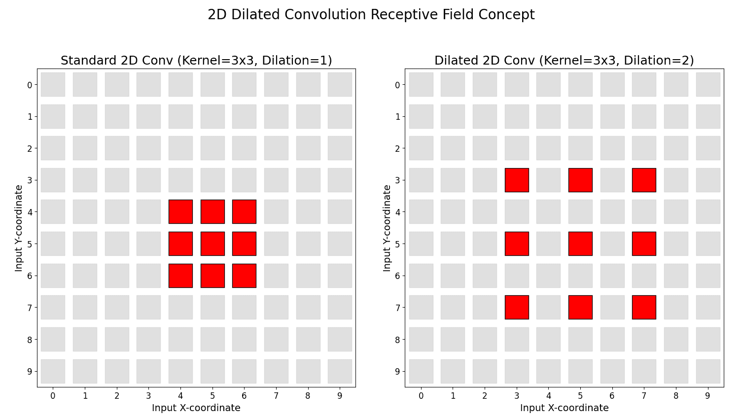
Reduction in Complexity: Reduces attention computation and memory from $\mathcal{O}(n^2)$ to a lower bound depending on the sparsity pattern.
In dilated attention, the dot-product $QK^\top$ is computed only at dilated positions:
$\mbox{Attention}_{\text{dilated}}(Q, K, V) = \mbox{Softmax}\left(\frac{QK_d^\top}{\sqrt{d_k}}\right) V_d$
Where:
$K_d, V_d$ are the dilated subsets of keys and values.
$d_k$ is the key dimension.
Below is the visualization of dilated attention with a dilation rate of 3.
Login to view more content
August 7, 2025
DL0028 Sliding Window Attention
Explain the sliding window attention mechanism in transformer architectures.
Answer
Sliding window attention is an optimization that addresses the scalability issues of the standard self-attention mechanism. It improves efficiency by limiting the attention scope of each token to a local, fixed-size window. This enables transformer models to handle longer sequences more effectively without a quadratic increase in computational resources. The trade-off is a potential loss of global context.
Purpose: Efficiently scale attention for long sequences by restricting each token’s attention to a fixed-size local window instead of the full sequence.
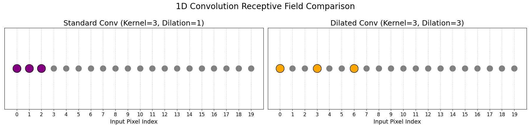
Window Size: Each token attends only to tokens within a fixed window of size $w$ (e.g., the token itself and $\pm \frac{w}{2}$ neighbors).
Sparse Attention: Results in a sparse attention matrix — reduces memory and computation from $\mathcal{O}(n^2)$ to $\mathcal{O}(n \cdot w)$ .
Here is a side-by-side comparison of Global Attention vs Sliding Window Attention: Each token attends to all others (dense matrix) in Global Attention. Each token attends only to a small window of nearby tokens (sparse band around the diagonal) in Sliding Window Attention.
Login to view more content
August 6, 2025
DL0024 Fixed-size Input in CNN
What is the “dilemma of fixed-size input” for CNNs? How is it typically resolved?
Answer
The “dilemma of fixed-size input” for Convolutional Neural Networks (CNNs) refers to the requirement that traditional CNN architectures demand input images of a predetermined, fixed size. This presents a challenge because real-world images often vary widely in dimensions.
Fixed Input Requirement: Traditional CNN architectures (like VGG or ResNet) require inputs of a fixed size due to the structure of fully connected layers at the end.
Data Preprocessing Constraint: Real-world images vary in size, so they must be resized or cropped, which may distort or lose important features.
Inefficiency & Information Loss: Resizing may stretch or compress content unnaturally, affecting model performance.
Below shows an example of information loss during resizing or cropping.

Common Solutions for the dilemma of fixed-size input:
(1) Global Average Pooling (GAP): Replaces fully connected layers, allowing input of variable size and reducing overfitting.
(2) Fully Convolutional Networks (FCNs): Use only convolutional and pooling layers, which can handle variable-sized inputs.
(3) Adaptive Pooling (e.g., in PyTorch): Pools features to a fixed size regardless of input dimensions.
Login to view more content
June 8, 2025
DL0023 Dilated Convolution
What are dilated convolutions? When would you use them?
Answer
Dilated convolutions enhance standard convolution by inserting gaps between filter elements, thereby allowing the network to gather more context (a larger receptive field) without an increase in parameters or a reduction in resolution.
Dilated convolutions (also known as atrous convolutions) modify standard convolution by inserting gaps (zeros) between kernel elements. A “dilation rate” dictates the spacing of these gaps. A dilation rate of 1 is a standard convolution.
Contrast with Pooling:
Pooling reduces spatial resolution (downsamples) while increasing the receptive field.
Dilated convolutions increase the receptive field without reducing resolution.
Multi-Scale Feature Extraction:
By adjusting the dilation rate, these convolutions can aggregate features from both local neighborhoods and larger regions, making it easier for the network to learn from multi-scale context.
Common Use Cases: Any task needing large receptive fields without downsampling.
(1) Semantic segmentation (e.g., DeepLab): Expand the receptive field and capture multi-scale context.
(2) Audio processing (e.g., WaveNet): Model long-range temporal dependencies.
Here is a 1D Dilated Convolution illustration.
Here is a 2D Dilated Convolution illustration.
Login to view more content
May 31, 2025
DL0019 Go Deep
How does increasing network depth impact the learning process?
Answer
Increasing network depth enhances feature learning and model power, but brings training instability, higher cost, and design complexity.
Increasing network depth can bring benefits:
(1) Improved Feature Hierarchy: Deeper layers can learn more abstract, high-level features. In image classification, early layers learn edges, deeper ones learn shapes and objects.
(2) Increased Model Capacity: More layers allow the network to model more complex functions and patterns.
(3) Improved Efficiency for Complex Functions: For certain complex functions, deep networks can represent them more efficiently with fewer neurons compared to shallow ones.
Increasing network depth can bring challenges:
(1) Vanishing/Exploding Gradients: Gradients can become extremely small or large as they propagate through many layers, hindering effective training, e.g., “Without techniques like skip connections, a 100-layer network might struggle to learn because gradients vanish before reaching early layers.“
(2) Increased Computational Cost (Challenge): Training deeper networks requires significantly more computational resources and time.
(3) Higher Data Requirements (Challenge): Deeper models have more parameters and are more prone to overfitting if not trained on large datasets.
The following example visually compares a shallow and a deep neural network on learning a complex function.
Login to view more content
May 30, 2025
DL0018 NaN Values
What are the common causes for a deep learning model to output NaN values?
Answer
NaN outputs in deep learning usually stem from unstable math operations, gradient issues, bad hyperparameters, or data problems. Prevent this with proper initialization, proper normalization, stable activation functions, and well-tuned hyperparameters.
Here are the common causes for a deep learning model to output NaN values:
(1) Exploding Gradients: Gradients become excessively large during training, leading to NaN weight updates
(2) Numerical Instability: Operations like log(0), division by zero, or square roots of negative numbers. Without a small constant (epsilon) in its denominator, batch normalization will suffer from division by zero if a batch has zero variance.
(3) Improper Learning Rate: Too high a learning rate can cause parameter updates to diverge and push model parameters to extreme values.
(4) Incorrect Weight Initialization: Incorrectly initializing all weights to very large positive numbers can cause activations to overflow immediately.
(5) Data Issues: Input data contains NaN or extreme values.
Login to view more content
May 30, 2025
DL0015 Cold Start
What is a “cold start” problem in deep learning?
Answer
The cold start problem is the difficulty of making reliable predictions for new entities (such as users, items, or contexts) lacking historical data.
Many deep learning models, especially in recommendation systems, rely on abundant past data to learn meaningful patterns. When a new user or item is introduced, the model struggles because it doesn’t have enough information to produce accurate predictions.
Mitigation Strategies for the Cold Start Problem:
(1) Transfer Learning / Pretrained Models: Use embeddings or models pre-trained on similar tasks to provide a starting point.
(2) Hybrid Recommendation Models: Combine collaborative filtering (CF) and content-based methods.
(3) Active Learning / User Onboarding: Actively gather more data for new entities through user interactions.
Login to view more content
May 26, 2025
DL0014 Mixed Precision Training
Can you explain the primary benefits of using mixed precision training in deep learning?
Answer
Mixed precision training accelerates deep learning by using both FP32 and FP16 operations, which reduces memory and computational requirements while maintaining model accuracy, resulting in faster and more efficient training.
(1) Faster Training: Uses lower-precision (e.g., FP16) operations on supported hardware (like GPUs/TPUs), which are faster than FP32.
(2) Reduced Memory Usage: Lower-bit representations decrease memory footprint, allowing larger batch sizes or models.
(3) Higher Throughput: More computations per second due to reduced precision, which can speed up training time.
(4) Supports Large Models: Enables training of models that wouldn’t fit in memory with full precision.
(5) Maintains Accuracy: With proper scaling (e.g., loss scaling), training stability and final model accuracy can typically be preserved.
Login to view more content
May 22, 2025
DL0013 Instance Normalization
Can you explain what Instance Normalization is in the context of deep learning?
Answer
Instance Normalization (IN) normalizes each individual data sample (often per channel) by subtracting its own mean and dividing by its variance, then applying a scale and shift. This makes it ideal for applications where per-instance adjustment is needed, such as artistic style transfer, ensuring that the normalization is not affected by the mini-batch composition.
Here are the equations for calculating Instance Normalization output $y_{nchw}$ for input $x_{nchw}$ :
$\mu_{nc} = \frac{1}{HW} \sum_{h=1}^{H} \sum_{w=1}^{W} x_{nchw}$
$\sigma_{nc}^2 = \frac{1}{HW} \sum_{h=1}^{H} \sum_{w=1}^{W} (x_{nchw} - \mu_{nc})^2$
$\hat{x}_{nchw}=\frac{{x}_{nchw} - \mu_{nc}}{\sqrt{\sigma_{nc}^2 + \epsilon}}$
$y_{nchw} = \gamma_c \hat{x}_{nchw} + \beta_c$
Where:
$x_{nchw}$ is the input feature at batch $n$ , channel $c$ , height $h$ , and width $w$ .
$H$ is the height of the feature map (number of rows per channel).
$W$ is the width of the feature map (number of columns per channel).
$\mu_{nc}$ is the mean of all spatial values in channel $c$ of instance $n$ .
$\sigma_{nc}^2$ is the variance of spatial values in channel $c$ of instance $n$ .
$\hat{x}_{nchw}$ is the normalized value after subtracting the mean and dividing by the standard deviation.
$\epsilon$ is a small constant added to the denominator to prevent division by zero and improve numerical stability.
$y_{nchw}$ is the final output after applying normalization and scaling.
$\gamma_c$ is a learnable scale parameter for channel $c$ .
$\beta_c$ is a learnable shift parameter for channel $c$ .
Login to view more content
May 22, 2025