DL0018 NaN Values

NaN outputs almost always trace back to numerical instability somewhere in the pipeline: unstable math operations, exploding gradients, an oversized learning rate, bad weight initialization, or corrupted input data. Once any parameter becomes NaN or Inf, the poisoning propagates through every subsequent layer, so the model’s outputs quickly become NaN everywhere.

(1) Exploding Gradients: Gradients grow without bound through many layers, producing weight updates so large that parameters overflow to Inf/NaN.
(2) Unstable Math Operations: , division by zero, or square roots of negative numbers yield Inf/NaN. For example, batch normalization divides by zero variance if a batch is constant and no is used.
(3) Improper Learning Rate: A learning rate that is too high makes parameter updates diverge, pushing weights to extreme values that overflow.
(4) Incorrect Weight Initialization: Initializing weights to very large values can overflow activations on the very first forward pass.
(5) Data Issues: Inputs containing NaN, Inf, or extreme unnormalized values inject invalid numbers directly into the computation graph.

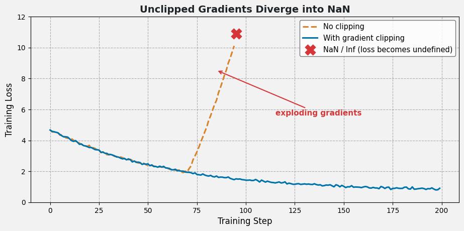
Figure 1: Unclipped gradients can explode within a few steps until the loss itself becomes NaN/Inf; gradient clipping keeps training on track.

NaN Loss vs NaN Outputs: The two are stages of the same instability. A NaN loss can even appear while model outputs are still finite. For example, cross-entropy computes , and a prediction extremely close to zero yields , which turns into NaN after the backward pass.

Figure 2: The five common causes and their standard fixes: every path ends at NaN parameters, hence NaN outputs.

Mathematical Formulation:

Where:

• is the predicted probability of the true class; without the clamp the loss diverges as approaches 0 and turns NaN in backprop.
• is the gradient vector and the clipping threshold; the second rule (norm clipping) caps update magnitude before gradients can overflow the parameters.