Tag: CNN

DL0195 Non-Max Suppression

What is Non-Max Suppression (NMS) in object detection, how does it work with confidence scores and IoU thresholds, and what are its limitations and alternatives such as Soft-NMS and DIoU-NMS?

Answer

NMS is the greedy post-processing step that turns a detector’s dense candidate set into a short, non-redundant list of boxes, and it normally runs independently per class. Boxes below a score floor are dropped first, the survivors are sorted by confidence, the highest-scoring box $M$ moves to the output list, and every remaining box whose IoU with $M$ exceeds a threshold $N_t$ is deleted. The loop then repeats on whatever is left: sort → pick the max → suppress → repeat. The algorithm rests on two assumptions, that confidence ranks localization quality and that a high IoU means two boxes describe the same object. Both fail in crowds, where the best box on a partially occluded neighbour can sit above $N_t$ against the winner and is silently erased. Soft-NMS replaces deletion with a monotonic score decay, and DIoU-NMS subtracts a normalized center distance from the IoU so that concentric duplicates are punished harder than offset neighbours.

(1) Greedy Per-Class Loop: NMS is not an optimizer, it is a sorted sweep, so the first mistake it makes is permanent because a deleted box never re-enters the pool.
(2) Two Thresholds, Not One: a score floor (often 0.001 for AP evaluation and 0.25 for a shipped product) plus the IoU threshold $N_t$ in the 0.5 to 0.7 range, with a top- $k$ cap in front to bound the cost.
(3) Confidence Is The Ranking Key: classification score and box quality are only loosely correlated, so NMS can keep a confident but sloppy box and delete a precise one, which is why IoU-aware or centerness-weighted scores improve NMS without touching the algorithm.
(4) Cost: an $O(n \log n)$ sort plus up to $O(n^2)$ pairwise IoU tests, which is why production stacks cap candidates and run a batched CUDA kernel.
(5) Dominant Failure Mode: a single global $N_t$ must serve sparse and crowded regions of the same image, so lowering it kills recall in crowds and raising it floods sparse regions with duplicates.
(6) Alternatives: Soft-NMS (linear or Gaussian decay), DIoU-NMS (center-distance penalty), Weighted and Cluster-NMS, Matrix NMS, and NMS-free detectors that learn one-to-one assignment instead.

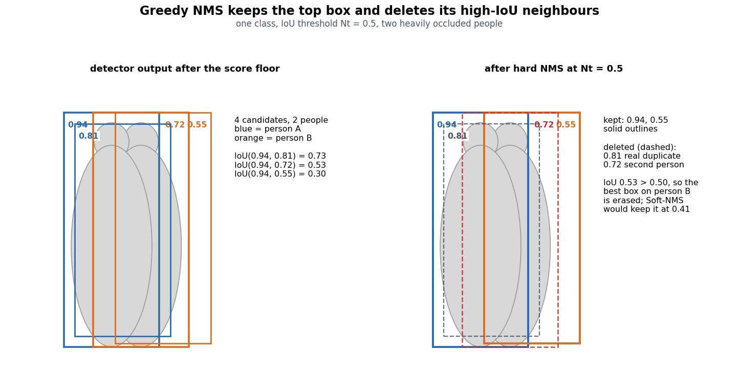
Two side-by-side panels showing a heavily occluded pair of pedestrians. The left panel draws four candidate boxes with confidence scores 0.94 and 0.81 on the first person and 0.72 and 0.55 on the second, with the pairwise IoU values against the top box listed. The right panel shows the result of greedy NMS at IoU threshold 0.5: the 0.94 and 0.55 boxes are kept as solid outlines while the 0.81 duplicate and the 0.72 box on the second person are drawn dashed and grey as suppressed.

Figure 1: Greedy NMS on a heavily occluded pair. The 0.81 box is a genuine duplicate and should go, but the 0.72 box is the detector’s best evidence for the second person, and its IoU of 0.53 with the winner crosses the 0.5 threshold, so hard NMS erases it. What remains for that person is a poorly localized 0.55 box, and Gaussian Soft-NMS would instead keep the 0.72 box at a decayed 0.41.

Mathematical Formulation:
$M = \arg\max_{b_i \in \mathcal{B}} s_i$
$\mathrm{IoU}(M, b_i) = |M \cap b_i| / |M \cup b_i|$
$s_i \leftarrow s_i \cdot \mathbf{1}[\mathrm{IoU}(M, b_i) \leq N_t]$
$s_i \leftarrow s_i \, (1 - \mathrm{IoU}(M, b_i))$
$s_i \leftarrow s_i \exp(-\mathrm{IoU}(M, b_i)^2 / \sigma)$
$\mathrm{DIoU}(M, b_i) = \mathrm{IoU} - \rho^2 / c^2$

Where:

$\mathcal{B}$ is the current candidate set for one class, $b_i$ a box in it with score $s_i$ , and $M$ the current maximum-score box that is moved to the output list $\mathcal{D}$ .
$N_t$ is the IoU threshold; line 3 is hard NMS, which zeroes (deletes) any box overlapping $M$ more than $N_t$ .
Line 4 is linear Soft-NMS, applied only when $\mathrm{IoU}(M, b_i) > N_t$ ; line 5 is Gaussian Soft-NMS, applied to every remaining box with no threshold at all.
$\sigma$ controls the decay width, typically $\sigma = 0.5$ ; a smaller $\sigma$ makes Soft-NMS behave more like hard NMS.
$\rho$ is the Euclidean distance between the two box centers and $c$ the diagonal of the smallest box enclosing both, so $\rho^2 / c^2$ lies in $[0, 1)$ and is scale-invariant.
$i$ indexes the surviving candidates, and the loop terminates when $\mathcal{B}$ is empty or every score falls under the final report floor.

Worked Decay For The Erased Box:
$\mathrm{IoU}(M, b) = 0.53 > N_t = 0.5$
$0.53^2 / 0.5 = 0.5618$
$0.72 \times \exp(-0.5618) = 0.41$

Hard NMS maps that box to 0, Soft-NMS maps it to 0.41, and the practical difference is whether a report threshold of 0.3 still shows the second person. This is also the clearest way to see why Soft-NMS buys roughly 1 to 2 AP on MS COCO with no retraining: average precision rewards a correctly located box even at low confidence, because a decayed detection is ranked below the confident ones and only costs precision after all the good detections are already counted. The same property is a liability in a live product, since nothing is ever deleted and the output list keeps every candidate at some non-zero score, so a final score floor and a top- $k$ cap become mandatory rather than optional.

Line chart with IoU against the kept box on the horizontal axis from 0 to 1 and the score multiplier applied to the overlapping box on the vertical axis from 0 to 1. Hard NMS is a step function that holds at 1 until IoU 0.5 and then drops to 0. Linear Soft-NMS holds at 1 until 0.5 and then falls linearly to 0 at IoU 1. Gaussian Soft-NMS with sigma 0.5 decays smoothly from 1 and reaches about 0.14 at IoU 1, with an annotation marking that IoU 0.53 keeps 57 percent of the score.

Figure 2: Every NMS variant is just a different score multiplier as a function of IoU. Hard NMS is a discontinuous step at $N_t$ , which is what makes a 0.499 and a 0.501 overlap have completely different fates. Soft-NMS swaps the step for a monotonic decay, so the cliff at the threshold disappears and the ranking, rather than a hard rule, decides what appears in the final list.

DIoU-NMS attacks a different weakness: IoU alone cannot tell a concentric duplicate from a genuinely different object. Two boxes that share a center almost certainly describe the same thing, while two boxes with the same IoU but far-apart centers are much more likely to be neighbouring instances, so the criterion becomes IoU minus the squared center distance normalized by the enclosing diagonal. The catch is that same normalization. For two tall, near-identical pedestrian boxes offset by a fraction of their width, $\rho^2 / c^2$ is on the order of 0.01, so DIoU-NMS behaves almost exactly like hard NMS on the case in Figure 1. It helps most where scale or center offset differs substantially, which is why it is usually reported together with the DIoU regression loss rather than as a standalone fix for crowds.

Two panels each showing a large kept box M with a candidate box. In the left panel the candidate is a smaller box concentric with M, both centers coincide, IoU is 0.25, the center distance is zero and DIoU stays 0.25 so the box is suppressed at a 0.20 threshold. In the right panel the candidate is the same size as M but shifted horizontally, IoU is again 0.25, the center distance is 3.6 with the dashed enclosing box diagonal marked, the penalty is 0.10 and DIoU falls to 0.15 so the box is kept.

Figure 3: Both candidates have identical IoU 0.25 with the kept box, so hard NMS treats them identically. DIoU-NMS separates them: the concentric box keeps DIoU 0.25 and is deleted, while the offset box pays a 0.10 penalty and survives at 0.15 under a 0.20 threshold. Because the penalty is divided by the enclosing-box diagonal, it only bites when the center offset is large relative to the pair’s extent.

Property	Hard NMS	Soft-NMS	DIoU-NMS
Rule on an overlapping box	Delete if IoU exceeds Nt	Multiply the score by a linear or Gaussian decay, never delete	Delete if IoU minus the normalized center distance exceeds the threshold
Hyperparameters	Nt only, usually 0.5 to 0.7	Decay form, sigma near 0.5, plus a mandatory final score floor	Threshold plus the implicit distance normalization (sometimes an exponent beta)
Output size	Bounded and small	Every candidate survives with some score, so top-k is required	Bounded, slightly larger than hard NMS
Crowded scenes	Worst case, deletes true neighbours outright	Best AP gain, roughly 1 to 2 AP on MS COCO with no retraining	Helps when centers differ; near no effect for side-by-side boxes of equal size
Cost	Sort plus pairwise IoU, fast batched CUDA kernel	Same order but no early deletion, so more IoU work and a longer output list	Hard NMS plus one center-distance term per pair
Typical use	Default in Faster R-CNN and YOLO inference paths	Benchmark AP, crowd and dense-object settings, offline pipelines	Shipped with the DIoU/CIoU loss family, for example YOLOv4

The deeper limitation is structural rather than parametric: NMS is a non-differentiable, hand-tuned rule bolted onto a learned model, so the network is never trained to produce exactly one box per object. That is what NMS-free detectors remove. DETR-style models use Hungarian one-to-one matching during training, so duplicate suppression becomes a learned property of the decoder, and YOLOv10 keeps a one-to-many head for training signal while using a one-to-one head at inference, eliminating the NMS stage and its latency variance entirely.

August 21, 2026

DL0194 Sensor Degradation Feature Extractor

How do you detect and handle sensor degradation (lens distortion, rain noise, sensor misalignment) dynamically within a deep feature extractor pipeline, for a production perception stack such as a robotaxi’s camera-LiDAR fusion model or a Valeo-style surround-view ADAS?

Answer

Degradation is not handled by making the backbone bigger. It is handled by a cheap monitoring path that runs beside the feature extractor and a policy layer that changes how the extractor’s outputs are consumed. Three monitor families are affordable per frame: referenceless image-quality and soiling heads on the raw or early-feature tensor, feature-space drift statistics such as a Mahalanobis distance between the current channel-mean vector and the training reference, and geometric self-consistency residuals such as cross-sensor reprojection error, which is the only signal that separates a genuine extrinsic shift from bad weather. Detection alone is worthless, so those signals drive three mitigations: a quality gate that reweights per-sensor features before fusion, FiLM-style conditioning that lets the shared trunk adapt its normalization to the measured degradation, and an operational-design-domain (ODD) fallback that reduces speed, disables a fused output, or triggers a wiper and an online extrinsic re-estimation. The pipeline therefore reads capture → ISP → undistort → backbone → gate → fusion → heads, with the monitors tapping the first three stages and writing only into the gate.

(1) Separate Detection From Correction: a small monitor head that answers “how bad is this input” is far easier to train and validate than a backbone expected to be silently invariant to everything. It also gives you an auditable signal to log.
(2) Three Complementary Signals: pixel-level quality catches soiling and droplets, feature drift catches global appearance shift like rain veiling or blooming, and reprojection residuals catch calibration error. No single one covers all three failure classes.
(3) Geometry For Geometry Faults: a 0.5 degree extrinsic yaw drift leaves every image looking perfectly clean, so appearance-based monitors are blind to it; only cross-sensor residuals or photometric alignment expose it.
(4) Gate The Fusion, Not The Backbone: down-weighting a corrupted branch with normalized weights $w_m$ is a one-line change at inference and needs no retraining, whereas swapping backbone weights per weather condition doubles the validation surface.
(5) Train For Dropout, Not Just For Rain: corruption augmentation plus random modality dropout is what makes a gated fusion model usable when a branch is masked, otherwise the fused head has never seen a zeroed input.
(6) Absolute Scores Plus An Abstention Path: a softmax gate can only express relative trust, so a separate calibrated absolute quality score must be able to declare that all sensors are bad and hand control to the ODD layer.

Architecture diagram with three sensor lanes for front camera, side camera, and LiDAR, each passing through a per-sensor encoder and a quality head, all feeding a tall degradation gate box that computes fusion weights and FiLM conditioning, then a feature fusion block, then detection heads and a degradation-state and fallback block, with an online monitor box at the bottom sending dashed arrows to the gate and back to the encoder for recalibration

Figure 1: The monitors sit outside the critical path and write only into the gate. An alarm changes the fusion weight $w_m$ , the FiLM conditioning, and the declared ODD, but it never edits backbone weights at runtime, which keeps the deployed model bit-identical and the failure behaviour testable.

Each monitor has a different latency and a different false-alarm profile. The soiling and quality head is a per-tile classifier over an early feature map, typically under 1 ms on an embedded accelerator, and it is the only monitor fast enough to drive a physical actuator such as a nozzle or a heater. Feature drift is computed from the channel means of a mid-level tensor against a reference mean and covariance collected on clean data, then smoothed by a CUSUM accumulator so that a single dark frame does not raise an alarm while a sustained shift does within a few frames. Reprojection residuals need matched features across overlapping fields of view or LiDAR points projected into the image, so they run at a lower rate over a sliding window of several seconds, which is acceptable because extrinsic drift from thermal expansion or a curb strike is either slow or a step change that persists. Lens distortion sits between these cases: an intrinsics change makes straight lines curve and inflates residuals even for a single camera, and the correct response is to re-estimate the undistortion look-up table rather than to touch the network, because a CNN trained on rectified images treats a mis-rectified frame as out-of-distribution geometry.

Two stacked time-series panels over 300 camera frames. The top panel shows feature-drift distance rising from about 1.15 to 3.5 during a shaded rain burst between frames 90 and 170 while the reprojection residual stays near 0.35 pixels, then a second shaded region after frame 200 where the reprojection residual steps to about 2.5 pixels while feature drift stays low, with a dashed one-pixel residual threshold. The bottom panel shows the CUSUM statistic on feature drift staying at zero, then sawtoothing above a threshold of five during the rain burst with alarm markers.

Figure 2: The two monitors have orthogonal signatures. Rain moves the feature-drift statistic and leaves the reprojection residual untouched, while a mount shift moves the residual by 2.5 px without disturbing appearance statistics at all. Reading only one monitor guarantees you misdiagnose one of the two faults.

Quality-Gated Fusion:
$q_m = \sigma(g_{\phi}(F_m))$
$\hat{F}_m = \gamma(q_m) \odot F_m + \beta(q_m)$
$w_m = \frac{\exp(a_m + \log q_m)}{\sum_j \exp(a_j + \log q_j)}$
$F = \sum_m w_m \hat{F}_m$

Where:

$F$ is the fused feature tensor consumed by the task heads, and $F_m$ is the raw feature map of sensor $m$ , with $\hat{F}_m$ its degradation-conditioned version.
$q_m \in [0,1]$ is the absolute quality score produced by a small monitor head $g_{\phi}$ with logistic output $\sigma$ ; it is supervised by synthetic corruption labels and calibrated on held-out real degraded clips.
$\gamma(\cdot)$ and $\beta(\cdot)$ are the FiLM scale and shift vectors, and $\odot$ is channel-wise multiplication.
$a_m$ is a content-dependent attention logit from the ordinary fusion module, so the gate combines what is informative with what is trustworthy.
$w_m$ sums to 1 over sensors $m$ , which is why a low but uniform $q$ across all sensors must be caught by the raw $q_m$ values rather than by the weights.

Runtime Degradation Monitors:
$d_t^2 = (\mu_t - \mu_0)^{\top} \Sigma_0^{-1} (\mu_t - \mu_0)$
$S_t = \max(0, S_{t-1} + d_t - k)$
$r_{ij} = \| u_i - \pi(T_{ij} X_j) \|_2$

Where:

$d_t$ is the Mahalanobis drift at frame $t$ between the current channel-mean vector $\mu_t$ of a mid-level feature map and the clean-data reference $\mu_0$ with covariance $\Sigma_0$ .
$S_t$ is the CUSUM statistic with slack $k$ , which is set just above the clean-condition mean of $d_t$ ; an alarm is raised when $S_t > h$ and $S_t$ is then reset to 0.
$r_{ij}$ is the reprojection residual in pixels for correspondence $(i,j)$ , where $u_i$ is the observed image point, $X_j$ the 3D point from LiDAR or a second camera, $T_{ij}$ the extrinsic transform, and $\pi$ the projection using current intrinsics.
A robust percentile of $r_{ij}$ above roughly 1 px sustained over a window indicates extrinsic or intrinsic drift rather than matching noise, and triggers online recalibration.

The handling policy has to be trained for, not bolted on. A gate that can zero a camera branch is only safe if the fused head saw randomly dropped modalities and heavy corruption augmentation during training, otherwise masking a branch pushes the fusion layer into a region it never visited and accuracy collapses harder than with the corrupted input left in place. Augmentation alone is also insufficient, because it buys average-case robustness while a gate buys graceful worst-case behaviour: at high rain severity the model that can lean on LiDAR keeps far more of its mAP than the model that must average a clean point cloud with a veiled image. The cost is roughly one mAP point in clean weather, from the gate occasionally distrusting a good camera, plus the engineering burden of calibrating $q_m$ so that the gate does not permanently learn to ignore a sensor after a single bad deployment week.

Line chart of mAP versus rain and spray severity from level zero to five for three configurations: a clean-trained fusion baseline falling from 58 to 19, the same model with corruption augmentation falling from 58 to 31, and augmentation plus quality gating with LiDAR fallback starting slightly lower at 57 and falling only to 40, with an annotation noting the gate down-weights the camera branch at high severity

Figure 3: Corruption augmentation flattens the curve, but only the quality gate changes the shape of the tail, because it can stop trusting the camera entirely. The 1-point clean-weather cost at severity 0 is the price of that option, and it is the number a reviewer should ask you for.

Degradation	Detection signal	Where it runs	Runtime mitigation
Lens soiling, droplets	Per-tile soiling mask, loss of high-frequency energy	Early feature map, per frame, under 1 ms	Actuate nozzle or heater, mask affected tiles, lower that camera’s weight
Rain, spray, fog veiling	Feature-drift CUSUM on channel statistics, quality head score	Mid-level tensor, per frame with a few-frame delay	FiLM conditioning, shift fusion weight toward LiDAR and radar
Intrinsics or distortion drift	Straight-line curvature, single-camera reprojection residual	Sliding window of seconds, off the critical path	Re-estimate the undistortion look-up table before the backbone
Extrinsic misalignment	Cross-sensor residual above 1 px, LiDAR edge to image edge offset	Sliding window, low rate, host CPU acceptable	Online extrinsic correction, disable geometric fusion if outside bound
Full blockage or frozen stream	Frame hash repetition, entropy collapse, timestamp gap	Driver layer, before the network	Drop the modality using dropout-trained fusion, reduce the declared ODD

August 21, 2026

DL0192 Depth Anything 3 Cross-View Depth Estimation

How does Depth Anything 3 enable cross-view interaction for consistent multi-view monocular depth estimation, and what architectural changes distinguish it from its single-view predecessors?

Answer

Depth Anything 3 keeps the monocular recipe of its predecessors and changes essentially one thing inside the network: the scope of self-attention. Each of the $N$ input views is patchified by the same plain DINOv2 encoder, the per-view token sequences are concatenated into a single sequence, and the stack then alternates between within-view attention, where a query sees only its own view and fine monocular detail survives, and cross-view attention, where every token attends to every token of every view and correspondence, relative pose, and a common scale are learned. No fusion module, cross-attention adapter, or cost volume is introduced. The pretrained attention weights are simply given a wider window, so a single-view input degenerates exactly to the original monocular model, which is why multi-view capability does not cost single-image quality. The second change is the output: instead of the per-image affine-invariant disparity of Depth Anything V1 and V2, DA3 predicts a depth-ray target per view (a depth map plus a ray map), and depth along predicted rays back-projects to one point cloud and one set of camera poses under a single global scale. That one target replaces the multi-head, multi-task output of VGGT-style geometry transformers, and the reported gains over VGGT are roughly 44% on camera pose accuracy and 25% on geometric accuracy, while monocular depth still improves over DA2.

(1) Attention Scope, Not A New Module: cross-view interaction is implemented by concatenating view tokens and letting the existing self-attention layers run over the union, so no modality-specific or view-specific parameters are added.
(2) Interleaved Within-View And Cross-View Layers: within-view layers protect high-frequency monocular detail, cross-view layers enforce geometric agreement, and the two are alternated through the stack.
(3) Input-Adaptive Degeneration: at $N = 1$ the cross-view layer is numerically identical to the single-view layer, so the model is a strict superset of its monocular predecessor rather than a compromise.
(4) Single Depth-Ray Target: one head predicts depth plus a ray map per view; depth along rays → point cloud, and camera pose is read out of the ray field instead of a dedicated pose head.
(5) One Global Scale For The Whole Set: normalization is fitted once over all views rather than a free scale and shift per image, which is precisely what removes per-frame flicker and non-overlapping point clouds.
(6) Plain Backbone, Teacher-Student Data: a vanilla DINOv2 transformer with a DPT-style dense head is enough; the accuracy comes from the target and from teacher-student pseudo-labelling, not from architectural specialisation.
(7) The Price Is Quadratic: a cross-view layer costs $N$ times a within-view layer, so view count, not image resolution, becomes the dominant memory term.

Architecture diagram: three input views feed one shared DINOv2 patch embedding that concatenates N times 1369 tokens into a single sequence, which passes through a within-view attention block and then a cross-view attention block interleaved over M blocks, then a shared DPT-style dense head that emits a depth map and a ray map per view, which are fused into one point cloud and camera poses in a shared frame under a single global scale

Figure 1: One encoder, two attention scopes, one target. The only cross-view machinery is the wider attention window, and the only output is a depth map plus a ray map per view, from which the point cloud and the camera poses are derived rather than predicted by separate heads.

It helps to look at the attention mask directly. With $N$ views of $L$ tokens each, a within-view layer is a block-diagonal mask: $N$ independent $L \times L$ blocks, exactly what a monocular model computes, repeated in parallel. A cross-view layer fills in the off-diagonal blocks, and those off-diagonal entries are the whole mechanism, because a token on a wall corner in view 3 can now match the same corner in view 1 and inherit its depth ordering. Because the projection matrices are unchanged, the same weights serve both scopes and the model never has to learn a separate matching operator. The cost of filling those blocks is the reason view count dominates the budget, and it is also the reason non-overlapping views buy nothing: the off-diagonal blocks exist, but there is no correspondence for them to find, so the relative scale between two disjoint clusters of views stays unconstrained.

Two 3-by-3 block attention masks for three views with eight tokens each: the left mask has only the three diagonal within-view blocks filled and the six off-diagonal blocks marked masked, totalling 192 token pairs; the right mask has the diagonal within-view blocks plus all six off-diagonal cross-view blocks filled, totalling 576 token pairs

Figure 2: The same layer, two masks. Single-view models compute only the block diagonal; DA3 fills the off-diagonal blocks, and cross-view correspondence lives entirely there. The pair count grows from $N L^2$ to $(NL)^2$ , a factor of exactly $N$ .

Mathematical Formulation:
$Z = [\,X_1; X_2; \ldots; X_N\,]$
$A_{\mathrm{within}}(v) = \mathrm{softmax}(Q_v K_v^{\top}/\sqrt{d})V_v$
$A_{\mathrm{cross}} = \mathrm{softmax}(QK^{\top}/\sqrt{d})V$
$P_v(u) = o_v + d_v(u)\, r_v(u)$
$s = \mathrm{median}_{v,u}\, \| P_v(u) \|$
$C_{\mathrm{within}} = N L^2$
$C_{\mathrm{cross}} = N^2 L^2$

Where:

$X_v \in \mathbb{R}^{L \times d}$ holds the tokens of view $v$ and $Z \in \mathbb{R}^{NL \times d}$ is the single concatenated sequence the transformer actually sees.
$Q_v, K_v, V_v$ are the projections restricted to one view, while $Q, K, V$ are the same projections applied to all of $Z$ ; the weights are shared, only the scope differs.
$u$ indexes pixels, $v \in \{1,\ldots,N\}$ indexes views, $L = (H/p)(W/p)$ is tokens per view for patch size $p$ , and $d$ is the model width.
$d_v(u)$ is the predicted depth and $(o_v, r_v(u))$ the predicted ray map (origin and unit direction) expressed in a shared frame, so $P_v(u)$ is a 3D point in that frame and the camera pose follows from fitting $r_v$ .
$s$ is a single global scale estimated jointly over all views and pixels, replacing the per-image scale and shift used by affine-invariant monocular training.
$C_{\mathrm{within}}$ and $C_{\mathrm{cross}}$ count attention token pairs per layer, so their ratio is $N$ and the KV cache of a cross-view layer grows linearly in $N$ .

Token Budget At 518 Pixels And Patch Size 14:
$L = 37 \times 37 = 1369$
$N L = 32 \times 1369 = 43808$
$C_{\mathrm{within}} = 32 \times 1369^2 \approx 6.0 \times 10^{7}$
$C_{\mathrm{cross}} = 43808^2 \approx 1.92 \times 10^{9}$

Thirty-two views at a modest resolution already put nearly 44k tokens in one sequence, and a single cross-view layer touches about 1.9 billion token pairs against 60 million for a within-view layer. This is why the interleaving ratio is a real design knob rather than a detail: every cross-view layer you insert buys consistency and pays $N$ times the attention cost, and it is why the practical deployment question for any-view geometry models is not accuracy but how many views fit on the device.

Log-scale line chart of attention token pairs per layer versus number of input views from 1 to 64, with a dashed blue line for a within-view layer growing linearly as N times L squared and a solid orange line for a cross-view layer growing quadratically as N L squared, annotated at N equals 32 with 43808 tokens and 1.92 billion versus 60 million pairs, and a note that the two curves coincide at N equals 1

Figure 3: Consistency is not free. A within-view layer scales linearly in view count while a cross-view layer scales quadratically, and the two curves meet at $N = 1$ , which is the formal statement of the input-adaptive property that keeps monocular quality intact.

The target change matters as much as the attention change. A per-image affine-invariant prediction is ambiguous by construction: two frames of the same room can be individually excellent and still disagree by a factor of two in scale, so stitching them produces a doubled wall. Fitting one scale over the whole view set turns depth from a per-image ranking problem into a set-level geometry problem, and the ray map supplies the missing piece by encoding where each pixel’s viewing ray points in the shared frame. Camera intrinsics and extrinsics then fall out of the ray field by a least-squares fit rather than from a separate pose head, which is the concrete sense in which DA3 collapses a multi-task output into a single one.

Property	Depth Anything V1 / V2	VGGT	Depth Anything 3
Input	One image, independently per frame	A set of images in one forward pass	1 to N views, optionally with known poses
Cross-view mechanism	None; consistency is a post-processing problem	Alternating frame-wise and global attention with dedicated camera tokens	Interleaved within-view and cross-view self-attention, no new parameters
Prediction target	Affine-invariant relative disparity	Separate heads for camera, depth, point map, tracking	A single depth-ray target per view
Scale handling	Free scale and shift per image	Set-level, anchored to the first camera	One global scale fitted over the whole view set
Camera pose	Not produced	Predicted by a dedicated camera head	Read out of the predicted ray map
Backbone	DINOv2 ViT with a DPT dense head	ViT with specialised camera and register tokens	Plain DINOv2 ViT, no architectural specialisation
Dominant failure mode	Temporal flicker and misaligned point clouds across frames	Multi-task head interference and heavy memory	Quadratic cost in N; needs genuine overlap between views

August 20, 2026

DL0183 Anchor-Free vs Anchor-Based Detection

How do anchor-free object detectors such as FCOS, CenterNet, and CornerNet differ from anchor-based detectors such as Faster R-CNN and YOLOv3 in box parameterization, label assignment, and training stability?

Answer

The whole difference is what the regression head is measured against. An anchor-based head attaches $k$ prior boxes to every feature-map location and predicts four normalized deltas per prior, so a predicted box only exists relative to a tiled prior whose scales and aspect ratios were chosen in advance from dataset statistics. An anchor-free head has no prior: FCOS predicts the four positive distances from a location to the sides of the object it belongs to, while CornerNet and CenterNet predict heatmap peaks (two corners, or one center) plus a small size and offset regression read off at the peak. Because the reference disappears, the matching rule must change too, so IoU thresholds against priors are replaced by spatial containment plus a per-level size range, and modern detectors replace both with prediction-aware dynamic assignment. Training stability shifts rather than simply improving: anchor-free heads drop the unbounded log-space targets and the anchor hyperparameters, but they need centerness or IoU-aware quality weighting, per-level normalization of the distance targets, and an explicit tie-break for locations that fall inside two objects.

(1) Reference Frame: Anchor-based regresses log-space deltas against a discrete prior set, while anchor-free regresses geometry directly in stride units from a location or a keypoint.
(2) Matching Rule: IoU thresholds are replaced by point-in-box containment, and object scale is routed by FPN level size ranges instead of by anchor size.
(3) Candidate Count: Removing $k=9$ priors per location cuts predictions per level by 9x, which changes the positive/negative ratio the loss has to survive.
(4) Hyperparameter Surface: Scales, aspect ratios, and two IoU thresholds collapse into one set of level ranges plus a center-sampling radius.
(5) Stability Mechanics: Bounded positive distances with a GIoU-style box loss are better conditioned than log deltas, but need per-level scaling or a learnable exponential to keep early gradients sane.
(6) Ambiguity Handling: Two overlapping objects can claim different anchors at the same location, whereas an anchor-free point must be broken by minimum-area assignment, and CenterNet simply collides when two centers land in the same output cell.

Three panels showing the same ground-truth box parameterized three ways: an anchor-based panel with a dashed prior box and an offset arrow to the ground-truth center plus log width and height deltas, an anchor-free panel with a single interior point and four arrows labeled l, t, r, b reaching the four sides, and a keypoint panel with Gaussian peaks at the top-left and bottom-right corners and at the box center with a width-height regression head

Figure 1: The same object, three parameterizations. The anchor head needs a matched prior before its four numbers mean anything, the dense point head predicts four positive distances that are meaningful on their own, and the keypoint head turns detection into peak localization plus a size read-out, so its only remaining prior is the output stride.

Mathematical Formulation:
$t_x = (x - x_a) / w_a$
$t_y = (y - y_a) / h_a$
$t_w = \log(w / w_a)$
$t_h = \log(h / h_a)$

Anchor-Free Distances And Centerness:
$l = (p_x - x_1) / s$
$t = (p_y - y_1) / s$
$r = (x_2 - p_x) / s$
$b = (y_2 - p_y) / s$
$c_x = \min(l,r) / \max(l,r)$
$c_y = \min(t,b) / \max(t,b)$
$c = \sqrt{c_x c_y}$

Where:

$(x,y,w,h)$ is the predicted box and $(x_a,y_a,w_a,h_a)$ the matched anchor, so the four deltas are undefined without an assignment step.
$(t_x,t_y,t_w,t_h)$ are the anchor-based targets; the logarithm makes size ratios additive and keeps targets near zero when the prior already fits, but it is unbounded on both sides for a badly matched prior.
$p = (p_x, p_y)$ is the image-space center of a feature location and $s$ its level stride, typically 8 up to 128 across P3 to P7.
$(x_1,y_1,x_2,y_2)$ are the ground-truth corners; requiring all four of $l, t, r, b > 0$ is exactly the point-in-box positive test that replaces the IoU threshold.
$c \in (0,1]$ is centerness, multiplied into the classification score at inference so boxes regressed from near an object border are down-ranked before NMS.
A point is routed to level $j$ only if $\max(l,t,r,b)$ falls inside that level’s size interval $(m_{j-1}, m_j)$ , which is the anchor-free replacement for choosing anchor scales.

Assignment is where the two families really diverge. Faster R-CNN and YOLOv3 label a prediction by measuring IoU between a fixed prior and the ground truth, which needs a positive threshold, a negative threshold, an ignore band in between, and a rescue rule so every object keeps at least its best anchor. FCOS labels by geometry alone, then narrows the positive set with center sampling (only points within a radius of a few strides from the object center), which raises average positive quality without touching IoU at all. Keypoint methods go further and effectively skip matching: CenterNet splats a Gaussian at the object center on a stride-4 heatmap and treats the single peak cell as the only positive, which is why it needs no NMS but breaks when two centers quantize to the same cell. The lineage since then is a steady handover of the assignment decision from hand-set priors to the model itself: fixed anchors → dense point containment → adaptive statistics in ATSS → prediction-aware costs in SimOTA and TOOD.

Three 12 by 8 feature grids with the same ground-truth box overlaid. The first grid shows dashed anchor boxes of three aspect ratios at one cell and twelve shaded positive cells selected by an IoU threshold. The second grid shades all twenty cells whose centers fall inside the box in light gray and highlights the central three by three block kept by center sampling. The third grid highlights six irregularly placed cells chosen by a prediction-aware cost.

Figure 2: One box, three positive sets. IoU matching scores 9 anchors per cell and keeps a handful, so the imbalance is roughly 1:71 here; center sampling keeps 9 of 96 points with no IoU computation at all; dynamic top-k chooses a variable number of positives from the model’s own cost, which removes thresholds but makes the label set change as training proceeds.

Candidate Count On A RetinaNet-Style FPN (800 x 1024 Input):
$12800 + 3200 + 800 + 208 + 56 = 17064$
$A_{\mathrm{anchor}} = 9 \times 17064 = 153576$
$A_{\mathrm{free}} = 17064$

The count explains most of the practical differences. With about 154k anchors and a few dozen positives per image, an anchor-based one-stage head lives or dies on focal loss or a mined 1:3 negative ratio, and it pays memory and time for an IoU matrix between every anchor and every ground-truth box. Dropping to 17k points removes that matrix, cuts head parameters by the same factor, and makes the box branch predict bounded, strictly positive quantities that pair naturally with an IoU or GIoU loss instead of a smooth-L1 on log deltas. The cost is that scale and ambiguity handling become explicit design choices: level size ranges decide which stride sees an object, and a point inside two boxes is assigned to the smaller-area ground truth, a rule that still degrades on heavily nested or crowded scenes.

Property	Anchor-based (Faster R-CNN, YOLOv3)	Anchor-free dense point (FCOS, ATSS)	Keypoint (CenterNet, CornerNet)
Box parameterization	Four deltas per prior, width and height in log space	Four positive distances to the sides, in stride units	Heatmap peak plus regressed size and sub-pixel offset
Positive assignment	IoU above 0.5 to 0.7, ignore band, best-anchor rescue	Point inside the box, narrowed by center sampling	Exactly one peak cell per object, Gaussian-weighted focal loss
Scale handling	Anchor scales and aspect ratios per level, tuned on the dataset	FPN level size ranges on max(l, t, r, b)	Single high-resolution stride-4 map, no level routing
Candidates per image	About 154k for 9 anchors on P3 to P7	About 17k, one prediction per location	One 200 x 256 heatmap per class
Quality calibration	Objectness or class score, optionally IoU prediction	Centerness or IoU branch multiplied into the score	Peak value itself acts as the confidence
Duplicate removal	NMS, mandatory because many priors fire per object	NMS, since several nearby points stay positive	3 x 3 max-pool peak extraction, no IoU-based NMS
Dominant failure mode	Unusual aspect ratios or tiny objects match no prior, so recall drops silently	Ambiguous points in overlapping boxes, resolved only by min-area	Two centers colliding in one stride-4 cell, or wrong corner grouping

August 20, 2026

DL0182 Semantic, Instance, and Panoptic Segmentation

What are the differences between Semantic, Instance, and Panoptic Segmentation, and when is each task formulation used in practice, for example inside an autonomous-driving perception stack?

Answer

The three tasks differ in what a label is allowed to be. Semantic segmentation assigns every pixel exactly one class out of $K$ and has no notion of object identity, so two touching cars collapse into a single connected “car” region. Instance segmentation does the opposite: it detects and masks each countable object separately with a confidence score, but it only covers thing classes, ignores amorphous stuff such as road, sky, and vegetation, and its masks may overlap each other or leave pixels uncovered. Panoptic segmentation is the union of the two: every pixel receives one pair $(c_p, z_p)$ of class plus instance id, stuff classes get a single segment with no id, things get one segment per object, and the output is a strict partition of the image with no overlaps and no unlabeled pixels except an explicit void region. Which formulation you pick follows the consumer of the output, not fashion. A planner that needs to count and track individual vehicles needs ids, whereas a free-space or sky-replacement module only needs a region mask.

(1) Label Space: semantic returns a class per pixel, instance returns a set of scored binary masks with classes, and panoptic returns a class plus an id per pixel.
(2) Things Versus Stuff: instance segmentation is defined only on countable things; semantic segmentation handles both but cannot separate two instances; panoptic handles both and separates instances.
(3) Overlap Constraint: instance masks are independent and can overlap, while panoptic forces a non-overlapping partition, which means any fusion of two heads must resolve conflicts explicitly.
(4) Metrics Differ In Kind: semantic uses mIoU, instance uses mask AP averaged over IoU thresholds and scores, and panoptic uses PQ at a single fixed matching threshold with no score sweep.
(5) Annotation Cost: stuff-only masks are cheap polygon paint, per-instance boundaries between adjacent same-class objects are the most expensive labels in the dataset.
(6) Practical Selection: use semantic for region questions, instance for counting and tracking, and panoptic when a downstream module needs one consistent scene interpretation per pixel.

Three panels showing the same toy scene of sky, road, two touching cars, and a person labeled three ways: semantic where both cars form one car region, instance where only the two cars and the person get scored masks that slightly overlap while sky and road are ignored, and panoptic where every pixel receives one class plus instance id with the two cars separated by a hard boundary

Figure 1: One scene, three label spaces. The interesting pixels are the ones on the boundary between the two touching cars: semantic segmentation is structurally unable to place that boundary, instance segmentation places it but may let the two masks overlap and says nothing about road or sky, and panoptic segmentation is required to place it and to label every remaining pixel exactly once.

In practice the formulation is chosen by the consumer. Free-space and drivable-area estimation, land-cover mapping from satellite imagery, portrait or sky matting, and organ or tumor delineation are region questions, so semantic segmentation is sufficient and its cheaper labels are a real advantage. Counting, tracking, and grasping are identity questions: counting cells in a microscopy image, tracking each pedestrian across frames, or picking one item out of a bin all require per-object masks, so instance segmentation (or its video extension) is the right task. Panoptic segmentation earns its extra cost when a single downstream consumer must be handed one coherent interpretation of every pixel, which is why it is the natural output format for driving perception and robot scene understanding, where the same map must answer both “is this pixel drivable” and “which vehicle is this”. A useful diagnostic question is whether two adjacent objects of the same class must ever be told apart. If the answer is no, panoptic annotation is money spent on a distinction nobody reads.

Mathematical Formulation:
$f_{\mathrm{sem}}(p) = c_p$
$f_{\mathrm{ins}} = \{(m_j, c_j, s_j)\}_{j=1}^{M}$
$f_{\mathrm{pan}}(p) = (c_p, z_p)$
$\mathrm{mIoU} = \frac{1}{K}\sum_{k=1}^{K}\frac{TP_k}{TP_k + FP_k + FN_k}$
$\mathrm{PQ} = \mathrm{SQ} \times \mathrm{RQ}$
$\mathrm{SQ} = \frac{1}{|TP|}\sum_{(g,q) \in TP}\mathrm{IoU}(g,q)$
$\mathrm{RQ} = \frac{|TP|}{|TP| + \frac{1}{2}|FP| + \frac{1}{2}|FN|}$

Where:

$p$ is a pixel, $c_p$ its class, and $z_p$ its instance id, which is undefined (shared) for stuff classes and unique per object for thing classes.
$K$ is the number of classes, split into disjoint thing and stuff subsets by the dataset definition rather than by the model.
$m_j$ is the $j$ -th predicted binary mask, $c_j$ its class, and $s_j$ its confidence; the $M$ masks are independent, so they may overlap and their union need not cover the image.
$TP$ , $FP$ , and $FN$ in PQ count segments, not pixels, with a ground-truth segment $g$ and a prediction $q$ matched when $\mathrm{IoU}(g,q) > 0.5$ ; that threshold makes the matching provably unique because panoptic segments cannot overlap.
$\mathrm{SQ}$ is segmentation quality, the mean IoU of matched pairs, and $\mathrm{RQ}$ is recognition quality, the F1 score over segments; PQ is reported per class and then averaged, and often split into $\mathrm{PQ}^{\mathrm{th}}$ and $\mathrm{PQ}^{\mathrm{st}}$ .
$TP_k$ in mIoU counts pixels of class $k$ , which is why mIoU is blind to how many objects a class region contains.

Worked Example (One Image):
$\mathrm{SQ} = 3.10 / 4 = 0.775$
$\mathrm{RQ} = 4 / (4 + 1 + 1) = 0.667$
$\mathrm{PQ} = 0.775 \times 0.667 = 0.517$

Four matched segments whose IoUs sum to 3.10 give an SQ of 0.775, and two false positives plus two false negatives each contribute a half count to the RQ denominator, so RQ is 0.667 and PQ lands at 0.517. The decomposition is the practically useful part: a high SQ with a low RQ means the masks are accurate but segments are being missed or hallucinated, which points at the classification and duplicate-removal path, while a high RQ with a low SQ means the right objects are found with sloppy boundaries, which points at output resolution and boundary supervision.

Diagram of panoptic quality computation with a left column of six ground-truth segments and a right column of six predicted segments, arrows joining four matched pairs labeled with IoU values 0.92, 0.81, 0.74 and 0.63, a red dashed pair at IoU 0.38 that fails the threshold and counts as both a false positive and a false negative, one unmatched ground-truth sky segment, one spurious truck prediction, and a side panel computing SQ 0.775, RQ 0.667 and PQ 0.517

Figure 2: PQ is a segment-level bipartite matching followed by a product of two interpretable factors. The pair at IoU 0.38 is the detail that separates candidates who have read the metric from those who have not: it is not a weak match, it is no match at all, and it is charged once as a false positive and once as a false negative.

Property	Semantic	Instance	Panoptic
Output per pixel	One class id	Zero, one, or several scored masks	Exactly one (class, instance id) pair
Stuff classes	Covered	Not part of the task	Covered as one segment per class
Separates same-class objects	No	Yes	Yes, and mandatory
Overlapping masks	Impossible by construction	Allowed and common	Forbidden, conflicts must be resolved
Standard metric	mIoU over pixels	Mask AP swept over IoU and score	PQ = SQ x RQ at IoU above 0.5
Classic architecture	FCN, DeepLab, per-pixel softmax	Mask R-CNN, box then mask head	Panoptic FPN, or mask-classification with queries
Typical use	Free space, land cover, matting, organ delineation	Counting, tracking, robotic grasping	Driving and robot scene understanding, one map for all consumers

August 20, 2026

DL0179 Grounding DINO vs Faster R-CNN

How does Grounding DINO’s open-vocabulary object detection, which conditions on free-form text, differ from classic Faster R-CNN’s closed-category detection in architecture, training data, and deployment flexibility?

Answer

Faster R-CNN is a closed-set detector: the label space is baked into a final linear layer of shape $(K+1) \times d$ , so the model can only ever emit one of the $K$ categories it was trained on plus background. Grounding DINO keeps the same output contract (boxes with scores) but deletes that fixed head and replaces it with a region-text similarity. A prompt such as “dog . traffic cone .” is encoded by BERT, its token features are fused with image features in three places (the neck feature enhancer, the language-guided query selection stage, and the cross-modality decoder), and each of the 900 decoder queries is scored by a dot product against every text token instead of by a softmax over classes. Because the class list moved out of the weight matrix and into the input, adding a category becomes a string edit rather than an annotation, retraining, and redeployment cycle. The bill arrives in training data (detection plus grounding plus caption-derived boxes instead of one boxed dataset) and in inference cost (a transformer detector with a text encoder instead of a ResNet with a two-layer head).

(1) Fixed Head vs Contrastive Alignment: Faster R-CNN classifies with $\mathrm{softmax}(W f_i + b)$ over $K+1$ rows; Grounding DINO scores each query against each text token and applies a sigmoid per pair, so categories do not compete for a shared probability mass.
(2) Text Is An Input, Not A Label Set: the prompt is runtime configuration, which means the same weights detect “forklift” today and “spilled pallet” tomorrow with no gradient step.
(3) Fusion Happens Early And Often: a late-fusion design that only compares final features would leave the proposal stage text-blind, so Grounding DINO injects language into the encoder, into query selection, and into the decoder.
(4) Detector Family Differs Too: anchors, RoIAlign, and NMS are replaced by DETR-style one-to-one Hungarian matching with learned queries, which removes the anchor and NMS hyperparameters but slows convergence.
(5) Training Data Is The Real Difference: COCO’s 80 categories over ~118k images versus a mixture of Objects365, GoldG, and caption-mined pseudo boxes covering tens of thousands of phrase types.
(6) Flexibility Costs Latency And Calibration: open-vocabulary scores are per-phrase and poorly comparable across phrases, so thresholds must be tuned per prompt rather than set once.

Side-by-side vertical pipelines: left panel shows Faster R-CNN with image only, ResNet-50 plus FPN, Region Proposal Network producing about a thousand proposals, RoIAlign with a two-FC box head, and a softmax over K plus one fixed classes followed by NMS; right panel shows Grounding DINO with two input lanes for image and text prompt, a Swin backbone and a BERT text encoder, a feature enhancer combining deformable self-attention with bi-directional image-text cross-attention, language-guided query selection producing 900 cross-modality queries, and a cross-modality decoder emitting region-text contrastive logits whose label space is the prompt

Figure 1: The vocabulary lives in a different place. On the left it is a row of $W$ ; on the right it is a string that enters the network beside the pixels, so language influences which regions are proposed at all, not only how a finished proposal is labeled.

The training recipe follows from that architecture. Faster R-CNN needs one homogeneous boxed dataset, and every category must appear with exhaustive box annotation, which is why closed-set benchmarks stall around a few hundred classes. Grounding DINO is trained on a mixture of supervision grades: fully annotated detection data (COCO, Objects365 with 365 categories), human phrase grounding data (GoldG, built from Flickr30k Entities and Visual Genome), and caption data whose boxes are pseudo-labeled by a teacher in the GLIP lineage. The reformulation that makes this legal is treating detection as grounding: a detection dataset is just a caption of concatenated category names, so a single per-token alignment loss (focal loss on region-token logits) consumes all three grades plus the usual $L_1$ and GIoU box terms. The payoff is that a Swin-T model reaches about 48.4 AP zero-shot on COCO without seeing a single COCO image, and roughly 27 AP on LVIS minival where the long tail is exactly what a fixed 80-way head cannot express.

Mathematical Formulation:
$p_i = \mathrm{softmax}(W f_i + b)$
$W \in \mathbb{R}^{(K+1) \times d}$
$s_{ij} = q_i^{\top} t_j$
$\hat{p}_{ij} = \sigma(s_{ij})$
$s_i(P) = \max_{j \in P} s_{ij}$

Where:

$p_i$ is the closed-set posterior for RoI $i$ over $K+1$ outcomes, and $f_i \in \mathbb{R}^{d}$ is its pooled RoIAlign feature; the row count of $W$ is the vocabulary, which is why the label space is a weight-shape decision.
$q_i \in \mathbb{R}^{d}$ is the $i$ -th decoder query (Grounding DINO uses $N_q = 900$ ) and $t_j \in \mathbb{R}^{d}$ is the $j$ -th projected text token feature; both are projected into one shared embedding space, so the dot product is directly the logit.
$\sigma$ is the sigmoid, so every region-token pair is an independent binary decision; nothing forces the scores of a query to sum to one across the prompt.
$P$ is the set of sub-word indices belonging to one phrase, and $s_i(P)$ is the phrase-level score obtained by taking the maximum over that phrase’s tokens.
Index ranges are $i \in \{1,\ldots,N_q\}$ and $j \in \{1,\ldots,L_t\}$ with $L_t \leq 256$ BERT sub-word tokens, which is the hard cap on how large a prompt vocabulary can be in one forward pass.

Two-panel figure: left panel is a grayscale bar chart of a Faster R-CNN softmax over person, car, dog, chair, tv, and background probabilities that sum to one, annotated that traffic cone has no column so mass is forced onto the nearest in-vocabulary class; right panel is a grayscale heatmap of sigmoid alignment scores between four decoder queries and the seven prompt sub-word tokens of dog . traffic cone . leash ., with high values where the cone query meets traffic and cone, the dog query meets dog, and the leash query meets leash, and near-zero values for the pavement query

Figure 2: Two different score semantics. The closed-set head must spend all probability mass inside its vocabulary, so an unseen object is mislabeled with confidence; the contrastive head gives each query an independent score per token, and a new phrase adds a column rather than a retrained row of $W$ .

Deployment flexibility is therefore real but not free. The prompt format matters: phrases are period-separated and Grounding DINO uses sub-sentence masking so unrelated category names do not attend to each other, yet cramming hundreds of categories into 256 tokens still degrades both accuracy and score calibration, and long or rare names fragment into sub-words whose max-pooled score behaves differently from a short common noun. Because $\hat{p}_{ij}$ is not normalized across phrases, a single global confidence threshold that is right for “person” is usually wrong for “loose cable”, so production systems keep a per-phrase threshold table. The common industrial pattern is not to serve the open-vocabulary model at all: use it plus a segmenter as an auto-labeler to bootstrap a dataset, then train or distill a fast closed-set detector for the frames-per-second and cost envelope the product actually needs.

Property	Faster R-CNN (closed set)	Grounding DINO (open vocabulary)
Label space	Rows of the classifier weight matrix, fixed at training time	Tokens of the prompt, chosen per request
Localization mechanism	Anchors, RPN proposals, RoIAlign, NMS at inference	900 learned queries, language-guided query selection, one-to-one Hungarian matching, no NMS
Classification	Softmax cross-entropy over $K+1$ classes	Focal loss on per-token region-text logits, sigmoid per pair
Training data	One exhaustively boxed dataset (COCO: 80 classes, ~118k images)	Detection (Objects365, 365 classes) plus grounding (GoldG) plus caption-mined pseudo boxes
Adding one category	Annotate, grow the head by about 5.1k parameters, retrain, revalidate, redeploy	Edit the prompt string, zero new parameters, no retraining
Reported accuracy	About 40 box AP on COCO with R50-FPN, undefined outside its 80 classes	48.4 AP zero-shot COCO and 57.2 AP fine-tuned with Swin-T; 52.5 AP zero-shot with Swin-L
Inference cost	Convolutional backbone plus a two-FC head, edge-deployable, easy to quantize	Transformer detector plus a text encoder; prompt features are cacheable when the vocabulary is fixed
Dominant failure mode	Confidently mislabels unseen objects as the nearest known class	Prompt-sensitive, per-phrase thresholds, degradation past the 256-token prompt budget

August 19, 2026

DL0164 BEV Transformation: Lift-Splat-Shoot

Explain Bird’s-Eye-View transformation methods such as Lift-Splat-Shoot and transformer cross-attention for mapping multi-view camera video into a unified 3D world representation, as used in camera-only autonomous driving stacks and benchmarked on nuScenes.

Answer

A BEV transformation converts $N_{c}$ perspective images, each of which has thrown away the depth of every pixel, into a single metric grid in the ego frame where one cell always means the same physical patch of ground. Every method must invent the missing depth, and the two families differ only in which direction they move information. Forward projection, introduced by Lift-Splat-Shoot (LSS), predicts a categorical depth distribution per pixel, lifts each pixel into a frustum of $D$ candidate 3D points weighted by that distribution, then splats the points into BEV pillars with sum pooling. Backward projection, popularised by BEVFormer, starts from a fixed set of learned BEV queries, projects each query’s 3D anchor points into every camera using the known intrinsics and extrinsics, and pulls features back with deformable cross-attention so no explicit depth prediction is required. Both produce the identical output contract, typically a $200 \times 200 \times 256$ feature map at roughly 0.5 m resolution, which is why detection, map segmentation, occupancy and planning heads can be shared, and both add temporal fusion by warping the previous BEV feature into the current ego frame before merging.

(1) The Core Difficulty Is Depth, Not Geometry: the pixel-to-ray mapping $K^{-1}$ and the camera-to-ego rigid transform are exactly known, so the only unknown is the scalar range along each ray.
(2) Forward Projection (Push): LSS predicts $\alpha_{u,v,d}$ over $D$ discrete depth bins, takes an outer product with the context feature, and voxel-pools the resulting frustum point cloud into pillars.
(3) Backward Projection (Pull): BEV queries carry their own 3D position, project into the cameras that actually see them, and sample features with deformable attention, which sidesteps depth estimation entirely.
(4) Shared Output Contract: both write into the same ego-frame grid, so the transformation is a swappable module rather than an architecture commitment.
(5) Temporal Recurrence Is Not Optional: warping $B_{t-1}$ by the ego pose delta and fusing it into $B_{t}$ is what makes velocity estimation and short-occlusion memory possible from cameras alone.
(6) Depth Supervision Decides Accuracy: BEVDepth showed that supervising $\alpha$ with LiDAR-projected depth, rather than letting the detection loss shape it, is the single largest quality lever for the forward family.

Pipeline diagram: six surround cameras feed a shared 2D backbone with FPN, which splits into a top lane predicting a per-pixel depth distribution over 59 bins followed by an outer product and voxel pooling of roughly one million frustum points, and a bottom lane of learned 200 by 200 BEV queries whose 3D anchors are projected into the hit cameras for deformable cross-attention over image features used as keys and values; both lanes write into one 200 by 200 by 256 unified BEV feature map that feeds detection, map and occupancy heads

Figure 1: Two directions, one destination. The push lane commits to a depth distribution and scatters features outward; the pull lane keeps the grid fixed and gathers features inward. Everything downstream of the unified BEV feature map is identical, which is why these modules are interchangeable in practice.

The forward path is best understood as a soft, differentiable version of unprojecting a depth map. A pixel with context feature $c_{u,v} \in \mathbb{R}^{C}$ does not pick one depth; it spreads that feature over all $D$ bins in proportion to $\alpha_{u,v,d}$ , so a confident pixel deposits nearly all of its mass in one pillar while an ambiguous pixel smears a faint trail along its ray. Because the splat is a sum, the operation is permutation-invariant and handles overlapping camera fields of view for free, and because it is differentiable, gradients reach the depth head through the pooling. The engineering cost is the frustum point count, which is why production implementations replace the naive scatter with a sorted cumulative-sum pooling kernel or a preallocated BEVPoolv2 index table that skips materialising the point cloud at all.

Three panels: a grid of image pixels with one highlighted pixel carrying a 256-dimensional context feature; a bar chart of the predicted probability over 59 depth bins showing a sharp peak near 18 metres for a confident pixel and a broad dashed curve for an ambiguous pixel; and a top-down bird's-eye-view grid with the camera at the origin, a ray fanning outward, circles along the ray whose size is proportional to the depth probability, and one highlighted 3 by 3 metre pillar where the points are sum-pooled

Figure 2: One pixel becomes $D$ weighted 3D points. The width of the depth distribution is literally the width of the smear in BEV, so a flat $\alpha$ over a textureless road or a night-time scene produces a long low-confidence streak instead of a localised object.

Forward Projection (Lift-Splat-Shoot):
$\tilde{u} = (u, v, 1)^{T}$
$p_{c} = d\, K^{-1} \tilde{u}$
$p_{e} = R\, p_{c} + t$
$F_{u,v,d} = \alpha_{u,v,d}\, c_{u,v}$
$\sum_{d=1}^{D} \alpha_{u,v,d} = 1$
$B(x,y) = \sum_{p \in \Pi(x,y)} F(p)$

Where:

$B(x,y) \in \mathbb{R}^{C}$ is the BEV feature at grid cell $(x,y)$ in the ego frame, and $\Pi(x,y)$ is the set of frustum points whose ego coordinates fall inside that pillar.
$\tilde{u}$ is the homogeneous pixel coordinate, $K$ the camera intrinsic matrix, and $(R, t)$ the camera-to-ego extrinsic rotation and translation.
$d$ indexes the depth bins, with $d \in \{1, \ldots, D\}$ over a fixed range such as 1 m to 60 m in 1 m steps, giving $D = 59$ .
$\alpha_{u,v,d}$ is the softmax depth distribution for pixel $(u,v)$ and $c_{u,v}$ its context feature, so $F_{u,v,d}$ is the outer-product lift.
The splat is sum pooling, which keeps the operation order-free across cameras and differentiable with respect to both $\alpha$ and $c$ .

The backward path inverts the flow of information. A query at grid cell $(x,y)$ is lifted to $N_{z}$ anchor heights along a vertical pillar, each anchor is projected into every camera, and only the cameras whose image plane actually contains the projection contribute. Deformable attention then samples a handful of learned offsets around each projected location, so cost scales with the number of queries rather than with image resolution times depth bins, and a query near a lane boundary can shift its sampling points to where the evidence is instead of trusting a predicted depth. The trade-off is that the geometry is now an attention prior rather than a hard constraint: if extrinsics are wrong, the network can still learn to compensate, which is convenient during training and dangerous during deployment because the failure is silent.

Backward Projection (Cross-Attention):
$q_{xy} = Q(x,y) + \mathrm{PE}(x,y)$
$r_{j} = (x, y, z_{j})$
$\hat{p}_{ij} = \pi_{i}(r_{j})$
$A_{i} = \sum_{j=1}^{N_{z}} \mathrm{DA}(q_{xy}, \hat{p}_{ij}, F_{i})$
$\mathrm{CA}(q_{xy}) = \frac{1}{|V_{xy}|} \sum_{i \in V_{xy}} A_{i}$

Where:

$\mathrm{CA}(q_{xy})$ is the cross-attention output written into BEV cell $(x,y)$ , and $q_{xy}$ is the learned query plus its 2D positional encoding.
$r_{j}$ is the $j$ -th pillar anchor at height $z_{j}$ , with $N_{z} = 4$ a common choice spanning roughly -5 m to 3 m.
$\pi_{i}$ is the full projection of camera $i$ , so $\hat{p}_{ij}$ is a sub-pixel image location and $F_{i}$ the multi-scale feature map of that camera.
$V_{xy}$ is the set of cameras whose frustum contains at least one anchor, so the average is taken only over hit views and empty views contribute nothing.
$\mathrm{DA}$ is deformable attention, which samples a few learned offsets around $\hat{p}_{ij}$ with bilinear interpolation instead of attending to all pixels.

Frustum Cost At A Typical Configuration:
$N_{pts} = N_{c} \cdot H \cdot W \cdot D$
$6 \times 32 \times 88 \times 59 = 996864$
$200 \times 200 = 40000$

Roughly one million frustum points collapse into forty thousand pillars, an average of about 25 points per cell, and that ratio is exactly why the pooling kernel rather than the backbone is often the latency bottleneck in the forward family. It also exposes the accuracy story: because every point sits on a known ray, a lateral mistake of one pixel at 50 m is only about 4 cm, while a 5% depth mistake at the same range is 2.5 m. BEV error is dominated by range error, and it grows linearly with distance.

Log-scale line chart of bird's-eye-view position error in metres against range from the ego vehicle from 2 to 80 metres, showing straight rising lines for 10 percent, 5 percent and 2 percent relative depth error, and a much lower line for a one-pixel lateral error at focal length 1266 pixels, with a dashed horizontal line at the 2 metre matching threshold and an annotation noting that a 5 percent depth error at 60 metres displaces the box by 3 metres

Figure 3: Range error, not image-plane error, sets BEV quality. A one-pixel lateral error stays under 10 cm across the whole working range, while a modest relative depth error crosses the 2 m matching threshold somewhere between 20 m and 100 m depending on the depth head, which is why depth supervision and long-baseline temporal stereo pay off so heavily.

Property	Forward push (LSS, BEVDet, BEVDepth)	Backward pull (BEVFormer)	Implicit 3D encoding (PETR)
Depth handling	Explicit categorical distribution over D bins, optionally LiDAR-supervised	No depth head; anchors at fixed pillar heights sample every hit view	3D coordinates baked into image position encodings, depth learned implicitly
Dominant cost	Frustum scatter of about 1M points; needs a cumsum or index-table kernel	40,000 queries times layers times sampling points, quadratic in grid side	Global attention over all image tokens, no explicit BEV grid to build
Calibration sensitivity	Hard geometric constraint, so extrinsic drift shifts features into wrong pillars	Attention can partly absorb drift, which hides the fault instead of surfacing it	Most tolerant, but least interpretable when a single camera goes bad
Temporal fusion	Warp and concatenate past BEV grids, or run temporal stereo across frames	Recurrent BEV self-attention on the ego-warped previous grid	Propagate sparse object queries forward in time, no grid to warp
Typical failure	Flat depth distribution smears a distant object along its ray	Empty cells still consume compute, and unseen regions hallucinate from priors	Weak spatial locality makes small distant objects easy to miss

August 19, 2026

DL0139 Multi-Camera Video VLM

How do multi-camera video VLMs fuse visual inputs across asynchronous camera feeds with overlapping fields of view, as in Waymo’s surround-camera perception stack?

Answer

Fusion is three separate problems solved in a fixed order: time alignment, per-view encoding, then spatial merging. Production rigs first put every camera on one clock (PTP or GPS-locked triggers) and stamp each frame with its own capture time, because software receive time is meaningless at 30 fps. Each view is then encoded independently by a weight-shared ViT and compressed to a small token set per frame, since the raw budget is multiplicative: 6 cameras at 8 frames of 256 tokens each is $12{,}288$ visual tokens before a single word of the prompt. The merge itself comes in two families. Token-level fusion concatenates all view tokens into one LLM context and tags each token with a camera-identity, extrinsic-pose, and timestamp embedding, letting attention discover the cross-view correspondence itself; this is the route taken by surround-view multimodal models such as Waymo’s EMMA. Geometric fusion instead defines 3D query points (BEV cells or object queries), projects each one into every camera using calibrated intrinsics and extrinsics warped by ego motion to a common query time, and merges the sampled features with per-camera weights, so a point seen by two overlapping cameras is fused once rather than described twice.

(1) One Clock Before Anything Else: hardware-triggered PTP or GPS sync plus a per-frame capture timestamp is the prerequisite; without it every downstream geometric step inherits an unknown offset.
(2) Shared Encoder Per View: one ViT with tied weights runs on all $N$ views, followed by token reduction (pooling, a Q-Former, or a perceiver resampler) to keep the context finite.
(3) Token-Level Fusion Is Implicit: concatenate everything and add camera-ID, pose, and time embeddings; flexible and calibration-tolerant, but the model must learn that two tokens describe the same object.
(4) Geometric Fusion Is Explicit: project each 3D query point into every camera and merge samples with confidence weights, which deduplicates the overlap region by construction.
(5) Asynchrony Is A Pose Problem: each view is warped by the ego transform between its own capture time and the query time $t_q$ , so odometry or IMU quality bounds fusion accuracy.
(6) Token Budget Dominates Cost: tokens grow as $N \cdot T \cdot P$ while self-attention grows as $O(L^2)$ , so doubling the camera count quadruples attention FLOPs.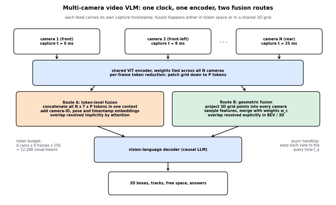
(7) Overlap Weighting Prevents Double Counting: weights derived from depth uncertainty and viewing angle favor the near, front-facing view over the oblique one.

The choice between the two families is not stylistic. Geometric fusion needs metric extrinsics, reasonable depth, and a rigid rig, and in exchange it gives a metrically consistent scene where 3D detection, tracking, and occupancy prediction are natural. Token-level fusion needs almost nothing beyond a camera index, survives loose or drifting calibration, and keeps the full appearance detail that a projection into a coarse BEV grid throws away, which matters for open-ended questions such as reading a sign visible in only one view. Most deployed stacks are hybrid: encode per view, warp features to a common timebase, lift to a shared 3D representation for the geometric heads, and pass a reduced token set of the same features into the language decoder for reasoning.

Top-to-bottom architecture diagram: three asynchronous camera feeds with different capture timestamps feed a shared ViT encoder with per-frame token reduction, which then branches into two fusion routes, token-level concatenation with camera-ID and pose embeddings on the left and geometric lifting into a shared BEV grid on the right, both feeding a vision-language decoder that emits text output

Figure 1: The pipeline is shared up to the fusion point: timestamped feeds → weight-tied ViT → token reduction, then either Route A (concatenate all tokens and let attention resolve the overlap) or Route B (project a 3D grid into every camera and merge with weights). Route A pays in context length, Route B pays in calibration and depth accuracy.

Mathematical Formulation:
$L_{vis} = N \cdot T \cdot P = 6 \cdot 8 \cdot 256 = 12288$
$\hat{X}_c = T_{c \leftarrow e}\, \Delta T(t_q, t_c)\, X_p$
$u_c = \pi(K_c\, \hat{X}_c)$
$B(p) = \frac{\sum_c m_c w_c\, F_c(u_c)}{\epsilon + \sum_c m_c w_c}$
$\Delta d = v\, |t_c - t_q|$
$\Delta d = 16.7 \cdot 0.025 = 0.42\ \text{m}$

Where:

$L_{vis}$ is the visual token count entering the decoder, with $N$ cameras, $T$ frames kept per camera, and $P$ tokens per frame after reduction.
$X_p$ is a 3D query point in the ego frame (a BEV cell center or a learned object query) and $\hat{X}_c$ is the same point expressed in camera $c$ ‘s frame at that camera’s own capture time.
$T_{c \leftarrow e}$ is the fixed extrinsic from ego to camera $c$ , and $\Delta T(t_q, t_c)$ is the ego-motion transform from the query time to the capture time, obtained from wheel odometry, IMU, or visual odometry.
$K_c$ is the intrinsic matrix, $\pi$ the perspective projection, $u_c$ the resulting pixel location, and $F_c(u_c)$ the encoder feature sampled there by bilinear interpolation.
$m_c \in \{0,1\}$ is the visibility mask (point inside the frustum and unoccluded), $w_c$ the per-camera confidence weight from depth uncertainty and incidence angle, and $\epsilon$ a guard so uncovered cells stay zero instead of dividing by zero.
$v$ is ego speed and $|t_c - t_q|$ the timestamp offset, so $\Delta d$ is the spatial error incurred by ignoring compensation; the numeric line uses $v = 16.7$ m/s (60 km/h) and a 25 ms offset expressed in seconds.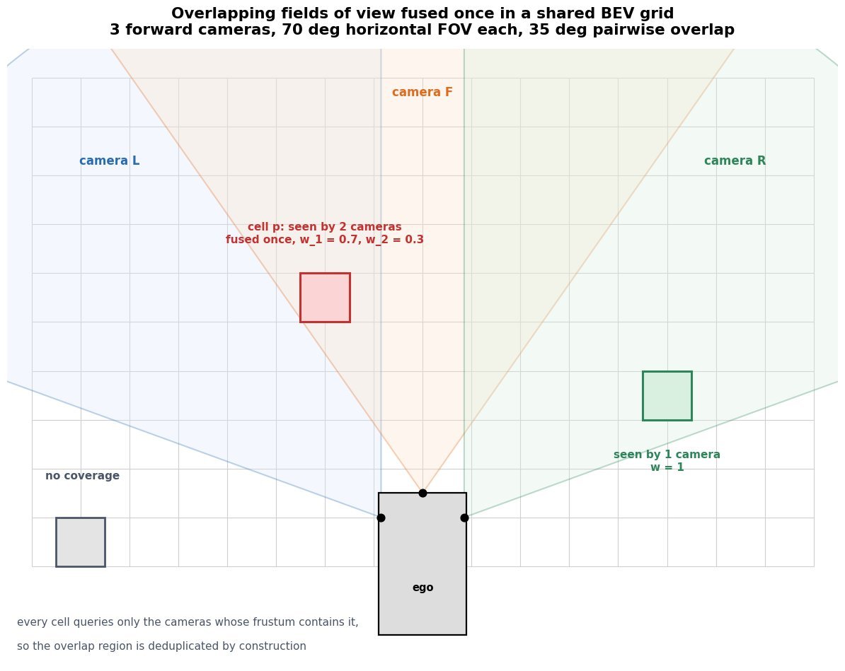

Top-down BEV diagram of an ego vehicle with three forward camera frustums drawn as shaded wedges that overlap pairwise, laid over a square BEV grid; one highlighted cell falls inside two wedges and is labeled as fused with two weights, another cell falls inside one wedge only, and a cell at the far left falls outside all wedges and is labeled as having no coverage

Figure 2: Why geometric fusion handles overlap cleanly. Each BEV cell queries every camera whose frustum contains it, so a cell in the pairwise overlap receives two samples that are averaged with confidence weights instead of appearing as two separate objects. Cells outside every frustum stay explicitly empty, which token-level concatenation cannot represent.

Asynchrony bites hardest at the selection step. With free-running 30 fps sensors, the newest available frame from each camera can be up to one full period old, so a naive “latest frame per camera” gather can mix captures spread across 33 ms. At 60 km/h the rig moves 0.55 m in that window, which is larger than the BEV cell size most stacks use, and the symptom is a smeared or duplicated object in the overlap region rather than an obvious crash. Two fixes are standard: warp features per view with $\Delta T(t_q, t_c)$ before sampling, and feed the residual offset to the model as a timestamp embedding so it can learn how much to trust a stale view. Hardware-triggered synchronous shutters remove the problem at the source and are worth the wiring cost on any rig that must produce metric output.

Left panel: timeline of four free-running 30 fps camera feeds with staggered capture phases, showing the newest frame available before a query time of 40 milliseconds for each camera and a double-headed arrow marking a 25 millisecond spread. Right panel: line chart of ego displacement in meters versus timestamp offset from 0 to 50 milliseconds for speeds of 10, 30, 60 and 100 kilometres per hour, with a dotted horizontal line at a 0.3 metre fusion tolerance

Figure 3: Free-running feeds mean the frames you gather at $t_q$ can span nearly a full frame period (left), and that spread converts directly into ego displacement (right). At highway speed even a 20 ms offset exceeds a typical 0.3 m fusion tolerance, which is why the ego-motion warp is not optional.

Property	Token-level concatenation	Dense BEV lifting	Sparse 3D queries
Shared representation	The LLM context itself, with camera-ID, pose and time embeddings	A metric BEV or voxel grid in the ego frame	A few hundred learned 3D queries with reference points
Overlap handling	Implicit; attention must learn that two tokens are one object	Explicit; one cell averages all cameras that see it	Explicit; one query attends to all views that contain its point
Asynchrony handling	Timestamp embedding only; residual error stays in the features	Ego-motion warp per view before sampling	Query propagation across frames with a motion-compensated pose
Calibration requirement	Low; a camera index and rough pose are enough	High; extrinsic drift of a degree visibly smears the grid	High for the projection, but errors stay local to each query
Cost scaling	Quadratic in N x T x P through self-attention	Linear in cameras, but grid resolution cubed in 3D	Linear in queries times cameras, cheapest at high N
Best for	Open-ended VQA, captioning, uncalibrated or ad hoc rigs	Occupancy, map and free-space prediction on a rigid rig	Streaming 3D detection and tracking under a latency budget

August 17, 2026

DL0124 3D Occupancy Flow

What is 3D Occupancy Flow? What is the tradeoff for predicting dense spatiotemporal occupancy grids instead of discrete 3D bounding-box trajectories?

Answer

3D Occupancy Flow is a joint perception-and-forecasting output format that replaces the list of tracked objects with a dense grid: for every voxel (or BEV cell) and every future waypoint the network predicts an occupancy probability plus a flow vector describing how the mass in that cell moves. Waymo’s Occupancy Flow Fields formulation predicts three quantities per waypoint on a $256 \times 256$ BEV grid covering roughly $80\ \text{m} \times 80\ \text{m}$ : observed occupancy, occluded occupancy, and backward flow. Camera-only 3D variants such as Occ3D on nuScenes predict a $200 \times 200 \times 16$ voxel grid at $0.4\ \text{m}$ resolution, and Tesla presented an occupancy network with an occupancy-flow head at its 2022 AI Day. The appeal is that free space and obstacle geometry become class-agnostic and non-parametric: a tipped-over mattress, an articulated trailer, a swinging crane boom, and an overhanging branch all get represented without appearing in a detector taxonomy, and probability mass can sit on both branches of a fork at once without a mode head or non-maximum suppression. The cost is that a grid has no notion of an object, so instance identity, track continuity, and per-agent attributes disappear, and the output tensor grows by roughly two orders of magnitude, which pushes cost onto compute, memory, label pipelines, and the loss function’s handling of a grid where the overwhelming majority of voxels are empty. In practice this is why most production stacks run occupancy flow alongside a box pipeline rather than as a drop-in replacement.

(1) Dense Spatiotemporal Output: the head emits $o_t(v)$ and $f_t(v)$ for every cell and every future timestep, not a parametric box with a heading and a velocity per agent.
(2) Class-Agnostic Geometry: anything that occupies space is representable, which removes the long-tail detection failure where an unlisted object class becomes invisible to the planner.
(3) Backward Flow, Not Forward: predicting motion from $t$ back to $t-1$ makes warping a gather with one source per cell, so mass never collides during the warp and a flow-grounded occupancy consistency check becomes well defined.
(4) Non-Parametric Multimodality: a grid holds several futures simultaneously as spread probability mass, but that same property makes averaged modes look like blur or ghost occupancy rather than a ranked set of hypotheses.
(5) Identity Is What You Give Up: without instance IDs, right-of-way logic, interaction-aware conditioning, and per-object intent signals such as turn indicators lose their handle on the scene.
(6) Cost Scales With The Grid: output size grows as $H W D T$ , dense labels require multi-sweep LiDAR accumulation and voxelization, and roughly 95% or more of voxels are empty, so class imbalance dominates the occupancy loss.

Diagram contrasting two forecasting pipelines from the same sensor input: an object-centric branch running detector, tracker, and trajectory predictor to emit sparse box waypoints, and an occupancy-centric branch running a BEV or voxel encoder with occupancy and backward-flow heads to emit a dense spatiotemporal grid

Figure 1: The object-centric branch (detect → track → forecast) produces a sparse, identity-carrying output limited by its taxonomy; the occupancy branch skips detection and data association entirely and produces a dense, class-agnostic grid with no instance IDs.

The deeper tradeoff is not really compute, it is what the downstream planner can express. A box trajectory is a commitment: this vehicle, with this ID, will be here in 3 seconds with this probability, which lets a planner reason about yielding to a specific agent, replay a scenario in simulation, and produce an auditable explanation for a maneuver. Occupancy flow is a statement about space, which is exactly what collision checking and drivable-free-space queries want, but a grid that hedges between “the cyclist goes straight” and “the cyclist turns” paints both corridors at moderate probability, and a naive cost function that treats any occupancy above a threshold as blocked yields the freezing-robot behavior. Occupancy flow partially recovers correspondence without identity: warping the previous occupancy along the predicted backward flow and multiplying it against the current occupancy gives a differentiable consistency term, so the model is penalized for teleporting mass even though it never names an object.

Mathematical Formulation:
$0 \leq o_t(v) \leq 1$
$\hat{o}_t = o_t \odot \mathcal{W}(o_{t-1}, f_t)$
$\mathcal{L} = \mathcal{L}_{occ} + \lambda \mathcal{L}_{flow}$
$\mathcal{L}_{occ} = \sum_{t=1}^{T} \sum_{v} \mathrm{BCE}(o_t(v), y_t(v))$
$\mathcal{L}_{flow} = \sum_{t=1}^{T} \sum_{v \in \Omega_t} \lVert f_t(v) - f_t^{*}(v) \rVert_1$
$N_{occ} = 200 \cdot 200 \cdot 16 \cdot 8 = 5.12 \times 10^{6}$
$N_{box} = 50 \cdot 6 \cdot 16 \cdot 5 = 2.40 \times 10^{4}$

Where:

$o_t(v)$ is the predicted occupancy probability of cell $v$ at future waypoint $t$ , and $f_t(v)$ is the backward flow vector pointing to where that mass sat at $t-1$ .
$\mathcal{W}$ is the warp operator that gathers $o_{t-1}$ along $f_t$ (bilinear or trilinear), and $\hat{o}_t$ is the flow-grounded occupancy used both as a loss term and as an evaluation metric.
$y_t(v)$ is the voxelized ground-truth occupancy label, $f_t^{*}$ the ground-truth flow, and $\Omega_t$ the set of genuinely occupied cells to which the flow loss is masked.
$t \in \{1, \ldots, T\}$ indexes waypoints and $v$ indexes the $H \times W \times D$ grid; $\lambda$ balances the two terms, and $\mathrm{BCE}$ is usually replaced by a focal or class-balanced variant because empty voxels dominate.
$N_{occ}$ counts predicted occupancy values for a $200 \times 200 \times 16$ grid over 8 waypoints, and $N_{box}$ counts a comparable box head with 50 agents, 6 modes, 16 waypoints, and 5 numbers per waypoint.
Required initial condition: $o_0$ and the whole grid must be expressed in the ego frame at $t = 0$ , so ego motion is compensated before flow is interpreted as agent motion.

Grid diagram showing occupancy at time t minus one in light dashed cells and predicted occupancy at time t in solid cells, with backward flow arrows drawn from each occupied cell at time t to the cell its mass came from, alongside the flow-grounded occupancy product equation

Figure 2: Backward flow assigns each occupied cell at time $t$ a single source cell at $t-1$ , so the warp is a gather rather than a scatter and the consistency product $o_t \odot \mathcal{W}(o_{t-1}, f_t)$ penalizes mass that appears without a plausible origin.

Resolution and horizon are the two knobs that make or break the design. Halving the voxel size multiplies the tensor by 8 in 3D, and every additional waypoint is another full grid, so a $0.2\ \text{m}$ grid over a 5-second horizon at $2\ \text{Hz}$ is far beyond a real vehicle compute budget once flow channels and semantics are added. Going the other way is not free either: at $0.4\ \text{m}$ voxels a pedestrian walking at $1.4\ \text{m/s}$ moves less than one voxel per $0.2\ \text{s}$ frame, so the flow target is sub-voxel and the occupancy channel alone cannot express the motion, which is precisely why the flow head is kept as a continuous regression rather than a discrete cell-to-cell assignment.

Log-scale bar chart of predicted output size per inference: 24000 numbers for multi-modal box trajectories, 524288 for a 256 by 256 BEV occupancy grid over 8 waypoints, 5.12 million for a 200 by 200 by 16 voxel grid over 8 waypoints, and 20.48 million once three flow channels are added

Figure 3: Output size is where the tradeoff becomes concrete: the 3D voxel grid predicts about 213x more numbers than a multi-modal box head, and adding a 3-channel flow field multiplies that by another 4 before any semantic classes are included.

Property	3D occupancy flow	Box trajectories	Hybrid stack
Output per inference	Millions of per-cell values, occupancy plus flow per waypoint	Tens of thousands of numbers, a few modes per tracked agent	Both, sharing one BEV or voxel backbone
Unlisted geometry	Represented, since occupancy is class-agnostic	Dropped if no detector class fits it	Covered by the occupancy branch
Instance identity	None; only flow-based correspondence	Explicit IDs, attributes, and track history	IDs from the box branch, geometry from the grid
Multimodality	Implicit in the probability field, no mode count to tune	Explicit ranked modes with confidences	Explicit modes for interaction, field for collision checks
Supervision	Accumulated multi-sweep LiDAR voxelized into dense labels	Human box and track annotations only	Both label pipelines must be maintained
Typical failure mode	Blurred or ghost occupancy that makes the planner over-conservative	Missed detection or ID switch removes an obstacle entirely	Disagreement between branches needs an arbitration policy

August 17, 2026

DL0117 3D Attention vs Frame Pooling

Compare 3D convolutional and space-time attention modules (e.g., TimeSformer) against frame-level pooling for temporal token aggregation in video encoders. When is each the right choice?

Answer

Both families turn $T$ frames of $N$ patch tokens into one clip representation, and they differ only in where temporal information is allowed to mix. Frame-level pooling runs a purely spatial encoder per frame and then averages or attention-pools the $T$ frame vectors (frames → per-frame ViT → pool → head), so no token ever sees another frame and the aggregation is permutation invariant over time. 3D modules mix earlier: a 3D convolution gives each token a local spatiotemporal receptive field of size $k_t$ , joint space-time attention lets all $NT$ tokens attend to each other, and TimeSformer’s divided space-time attention factorizes that into a temporal MSA over the same spatial position across frames followed by a spatial MSA inside each frame. The cost separation is the first thing to state in an interview: joint attention is $O(N^2T^2)$ in the pair count while divided is $O(N^2T + NT^2)$ , a ratio of $NT/(N+T)$ that reaches roughly 64x at 96 frames. The accuracy separation depends almost entirely on whether the label actually depends on frame order: on scene-biased Kinetics-400 dropping temporal attention costs about a point, while on Something-Something V2 the same ablation costs roughly 23 points.

(1) Pooling Is Order-Blind By Construction: mean or max pooling over frame embeddings is symmetric, so “opening a door” and “closing a door” produce the identical clip vector no matter how good the image backbone is.
(2) 3D Convolution Buys Locality Cheaply: cost is linear in $T$ , but the temporal receptive field grows only $k_t - 1$ frames per layer, so long-range order needs depth or a slow/fast dual pathway.
(3) Joint Attention Is Global But Quadratic: with ViT-B at 8 frames the token sequence is $196 \times 8 = 1568$ , and every added frame inflates the attention matrix quadratically.
(4) Factorization Is The Practical Default: divided space-time attention beat both space-only and joint attention in the TimeSformer ablations while being far cheaper than joint, which is why factorized variants dominate video ViTs.
(5) Benchmark Bias Decides The Verdict: appearance-biased datasets reward a strong image backbone, and temporally-ordered datasets punish any aggregator that discards order.
(6) Pooling Keeps System Properties Attention Destroys: per-frame embeddings can be cached, indexed, and streamed independently, which is why large-scale video retrieval still ships CLIP-style pooled encoders.

Three grids of tokens arranged as spatial patches by frames; in the first panel a query token connects only to tokens in its own frame, in the second it connects to its own frame plus the same spatial position in all frames, and in the third it connects to every token in the clip

Figure 1: The three aggregation schemes differ only in the attended set of a query token. Space-only attention plus pooling never crosses a frame boundary, divided space-time adds a one-dimensional temporal pass over the same spatial position, and joint attention connects all $NT$ tokens at quadratic cost.

A subtlety that separates mid from senior candidates is that divided attention is not simply “cheaper joint attention”. Its temporal MSA only compares a patch with the same spatial coordinate in other frames, so a fast-moving object that shifts several patches between frames is matched indirectly, through the spatial MSA that follows. That works because the two passes alternate at every block, but it is also why divided attention benefits from higher frame rates and larger patch strides, and why 3D convolutions with a spatial kernel remain competitive on motion-heavy, short-horizon tasks. Practically, inflating an image-pretrained ViT into a divided model requires zero-initializing the temporal projection so the network starts as an exact image model and the pretrained features survive the first epochs.

Mathematical Formulation:
$z = \frac{1}{T}\sum_{t=1}^{T} f(x_t)$
$C_{pool} = O(N^2 T D)$
$C_{3D} = O(k_t k_s^2 N T D^2)$
$C_{joint} = O(N^2 T^2 D)$
$C_{div} = O(N^2 T D + N T^2 D)$
$\frac{C_{joint}}{C_{div}} = \frac{NT}{N + T}$
$\frac{196 \cdot 96}{196 + 96} \approx 64$

Where:

$z$ is the clip embedding and $f$ the frozen or fine-tuned per-frame encoder applied to frame $x_t$ ; because the sum is symmetric, $z$ is unchanged by any permutation of the frames.
$t \in \{1, \ldots, T\}$ indexes frames, $N$ is the number of patch tokens per frame ( $196$ for ViT-B at $224 \times 224$ with patch 16), and $D$ is the model width.
$C_{pool}$ , $C_{joint}$ , and $C_{div}$ are the attention costs of space-only, joint space-time, and divided space-time blocks; all three exclude the identical per-token MLP term.
$k_t$ and $k_s$ are the temporal and spatial kernel sizes of a 3D convolution, whose cost is linear in $T$ but whose temporal receptive field after $L$ layers is only about $L(k_t - 1) + 1$ frames.
The ratio $NT/(N+T)$ holds whenever $T$ is at least 2; it grows toward $N$ as $T$ grows, so the saving is bounded above by the token count per frame.

Grouped bar chart of top-1 accuracy for space-only, joint space-time, and divided space-time attention on Kinetics-400 and Something-Something V2, showing a small gap on Kinetics and a very large gap on Something-Something

Figure 2: TimeSformer ViT-B ablations at 8 frames. Removing temporal mixing costs only 1.1 points on Kinetics-400, whose classes are largely identifiable from a single frame, but 22.9 points on Something-Something V2, where the label is defined by the direction of motion.

Property	Frame-level pooling	3D convolution (I3D, X3D, SlowFast)	Divided space-time attention
Temporal receptive field	None inside the encoder; one symmetric average at the end	Local, grows by k_t minus 1 frames per layer	Global over all T frames from the first block
Cost scaling in T	Linear, and trivially parallel across frames	Linear, with a constant factor of k_t	Linear plus a small quadratic term N T squared
Sensitive to frame order	No; shuffled clips give identical embeddings	Yes, within the local window	Yes, with temporal position embeddings
Image pretraining transfer	Perfect; the backbone is unchanged	Via kernel inflation and rescaling	Strong if the temporal projection is zero-initialized
Per-frame embedding caching	Yes; embeddings are reusable across clips and queries	No; features depend on neighboring frames	No; every block mixes across the whole clip
Typical failure	Collapses on reversible actions and counting tasks	Misses long-horizon structure without deep stacks	Weak on fast motion that leaves the shared patch column
Where it wins	Retrieval, tagging, zero-shot with image-text encoders	Short motion-heavy clips on constrained hardware	Order-sensitive recognition over dozens of frames

August 17, 2026