DL0023 Dilated Convolution

What are dilated convolutions? When would you use them?

Answer

Dilated convolutions (also called atrous convolutions) insert gaps between the elements of a convolutional kernel: with dilation rate d, the kernel samples every d-th input position instead of adjacent ones. This expands the receptive field without adding parameters and without reducing spatial resolution, a combination that pooling cannot offer. A dilation rate of 1 is just a standard convolution.

(1) Larger Receptive Field, Same Weights: A 3×3 kernel with dilation 2 covers a 5×5 area but still has only 9 weights.
(2) Resolution Preserved: Unlike pooling, dilation grows the receptive field while keeping the output the same size as a standard convolution, which is critical for dense prediction.
(3) Multi-Scale Context: Stacking or mixing dilation rates lets one network aggregate both fine local detail and broad context.

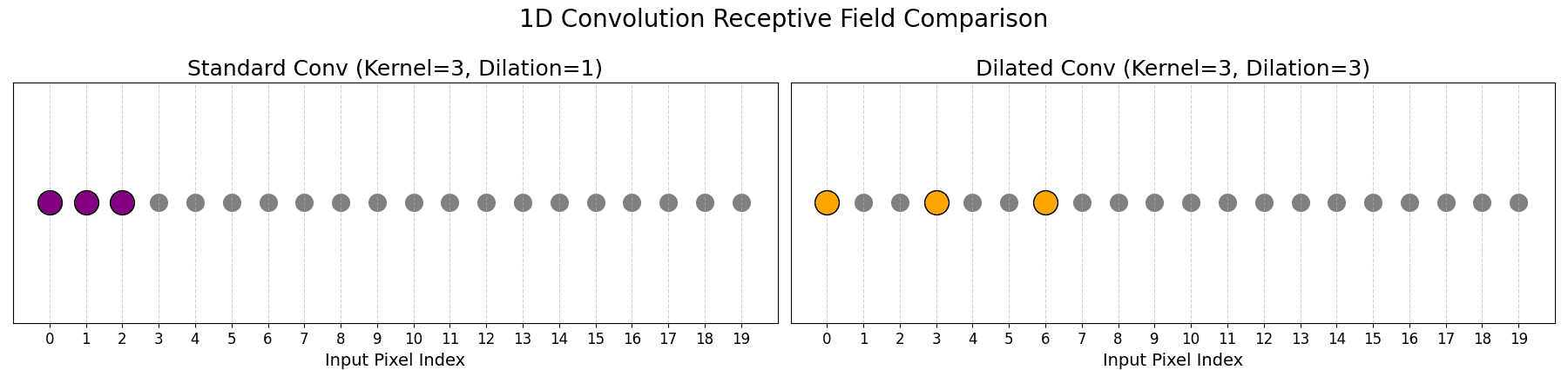
One-dimensional comparison of a standard kernel-3 convolution sampling three consecutive inputs versus a dilation-3 convolution sampling positions 0, 3, and 6 for a receptive field of seven with the same three weights.

Figure 1: Same 3 weights, wider view: dilation 3 spreads the taps across a receptive field of 7 instead of 3.

Mathematical Formulation:
y_{ij} = \sum_{a=1}^{k}\sum_{b=1}^{k} w_{ab}\; x_{i + d \cdot a,\; j + d \cdot b}
k_{eff} = k + (k - 1)(d - 1)

Where:

  • d is the dilation rate, the spacing between tapped positions (d = 1 is standard convolution).
  • k is the nominal kernel size; k_{eff} is the effective span of the dilated kernel (3×3 with d = 2 behaves like 5×5 with holes).
  • w_{ab} are the kernel weights; the parameter count is independent of d.

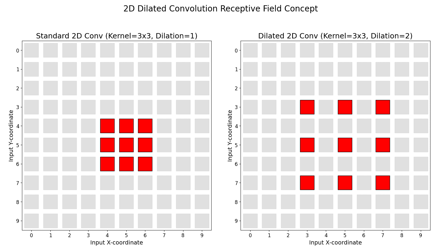
In Two Dimensions: The same idea applies to images: the kernel’s taps spread over a checkerboard-like stencil, expanding the covered span from 3×3 to 5×5 at dilation 2 while the channel count and output resolution stay unchanged.

Two ten-by-ten grids comparing a dense 3x3 standard convolution stencil against a sparse 3x3 dilation-2 stencil that spans a 5x5 region marked by a red dashed receptive-field box.

Figure 2: Dilation 2 turns a 3×3 stencil into a 5×5 receptive field (red dashed box), still only 9 multiply-accumulates.

When to Use Them: Any task needing large context at full resolution: semantic segmentation (DeepLab), audio generation (WaveNet models long-range temporal structure with exponentially growing dilation), and dense tasks like super-resolution or depth estimation.

Progression of a single input point through three stacked dilation-2 layers showing the response spreading into a checkerboard pattern with gaps between covered cells.

Figure 3: Gridding artifacts: stacking the same dilation leaves a checkerboard of unattended cells. Mitigate with hybrid dilation rates (e.g., 1, 2, 5) that overlap coverage.


Login to view more content


Log in to track your progress

Comments

Leave a Reply

Your email address will not be published. Required fields are marked *