Tag: KNN

  • ML0061 KNN and K-means

    What are the key differences between KNN and K-means?

    Answer

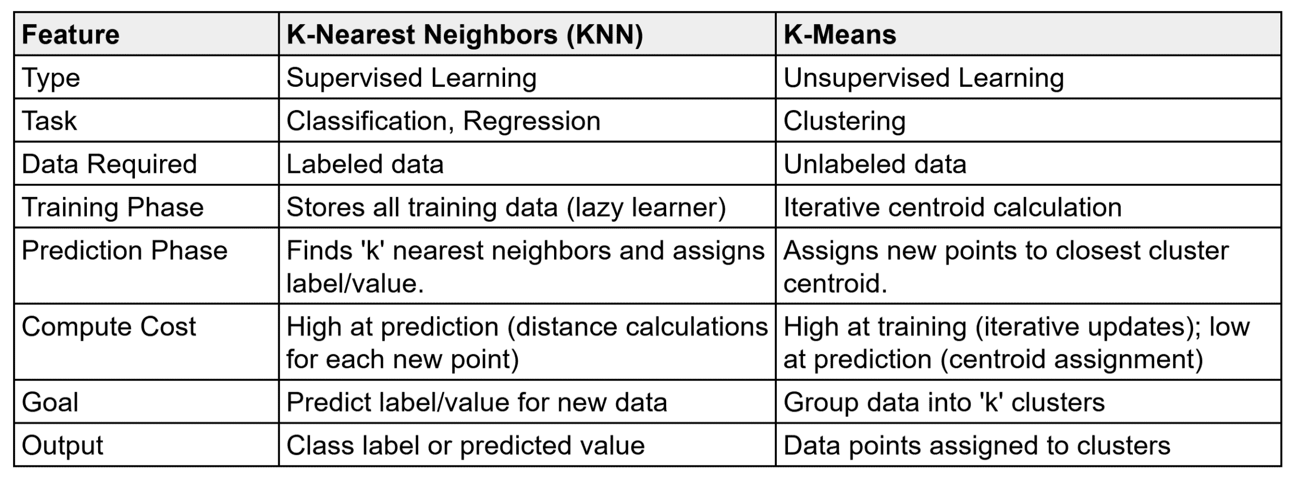
    KNN (K-Nearest Neighbors) is a supervised algorithm that classifies data using the labels of its nearest neighbors: prediction from historical labeled data. K-means is an unsupervised clustering technique that groups data purely by similarity, using no labels at all. Despite the shared “K”, they solve different problems.

    (1) Learning Type: KNN is supervised (classification/regression); K-means is unsupervised (clustering).
    (2) Objective: KNN predicts a new sample’s label from the majority vote (or average) of its K nearest neighbors; K-means partitions the dataset into K clusters by minimizing intra-cluster distance.
    (3) Training: KNN has no explicit training: it stores the entire dataset; K-means iteratively learns cluster centroids.
    (4) Prediction Cost: KNN is expensive at prediction (distance to every training point, sort, take the top K, then vote/average); K-means is cheap: distances to K centroids, assign the nearest.
    (5) Distance Use And Output: KNN uses distance to find neighbors and outputs a label or value; K-means uses distance to assign points to centroids and outputs cluster assignments plus centroids.

    FeatureK-Nearest Neighbors (KNN)K-Means
    TypeSupervised LearningUnsupervised Learning
    TaskClassification, RegressionClustering
    Data RequiredLabeled dataUnlabeled data
    Training PhaseStores all training data (lazy learner)Iterative centroid calculation
    Prediction PhaseFinds K nearest neighbors and assigns label/valueAssigns new points to closest cluster centroid
    Compute CostHigh at prediction (distance calculations for each new point)High at training (iterative updates); low at prediction (centroid assignment)
    GoalPredict label/value for new dataGroup data into K clusters
    OutputClass label or predicted valueData points assigned to clusters

    Mathematical Formulation:
    \hat{y} = \arg\max_{c \in \mathcal{C}} \; \sum_{i=1}^{K} \mathbb{1}(y_i = c)
    \min_{C_1, \ldots, C_K} \; \sum_{k=1}^{K} \sum_{x \in C_k} \|x - \mu_k\|^2

    Where:

    • KNN (first line): \hat{y} is the predicted class, \mathcal{C} the class set, y_i the label of the i-th nearest neighbor, and \mathbb{1}(\cdot) the vote-counting indicator.
    • K-means (second line): C_k is cluster k and \mu_k its centroid; the algorithm minimizes total within-cluster squared distance: no labels appear anywhere.
    Two panels on crescent moon data showing KNN separating the moons correctly while K-means cuts through them

    Figure 1: Same data, different goals: with labels, KNN’s local votes trace the two crescents perfectly (left); without labels, K-means can only split by nearest-centroid geometry and slices through both moons (right). KNN performs well here thanks to local decision-making; K-means fails because it assumes spherical clusters with linear boundaries.


    Login to view more content
  • ML0056 K Selection in KNN

    In the context of designing a K-Nearest Neighbors (KNN) model, can you explain your approach to selecting the value of K?

    Answer

    Selecting K in KNN is crucial because it directly controls model performance through the bias-variance tradeoff. The systematic approach is k-fold cross-validation combined with grid search over a range of K values, picking the one that minimizes validation error, informed where possible by domain knowledge and data characteristics.

    (1) Bias-Variance Tradeoff: A small K (e.g., 1) gives low bias but high variance: it tracks noise and overfits; a large K raises bias but lowers variance: it oversmooths and can underfit.
    (2) Use Odd Values For Classification: In binary classification, an odd K avoids tie votes.
    (3) Cross-Validation + Grid Search: Evaluate every candidate K with k-fold CV and select the minimizer of validation error.
    (4) Domain Knowledge: Prior knowledge of the data distribution can narrow the search range.

    Cross validated MSE curve over K from 1 to 20 with a minimum marked at K equals 4

    Figure 1: 5-fold CV error across K on a regression task: error dives as variance is tamed (tiny K overfits), bottoms at K = 4, then climbs steadily as over-averaging sets in (large K underfits). The minimizer is the selected K.

    Mathematical Formulation:
    CV(K) = \frac{1}{N} \sum_{i=1}^{N} \ell\big(y_i, \hat{y}_i(K)\big)

    Where:

    • y_i is the actual outcome for the i-th validation instance.
    • \hat{y}_i(K) is the prediction made using K neighbors (with the point’s own fold held out).
    • N is the number of validation samples and \ell the loss (e.g., squared error for regression, 0-1 for classification).

    Login to view more content
  • ML0055 KNN Regression

    Please explain how KNN Regression works.

    Answer

    K-Nearest Neighbors (KNN) Regression is a simple, instance-based algorithm that predicts a continuous output by finding the K nearest training points and averaging their target values. Its simplicity makes it easy to understand and implement, but performance is sensitive to K and the distance metric, and prediction is computationally expensive on large datasets since every query compares against all training samples. Like its classification sibling, KNN regression is a “lazy learner”: it builds no explicit model and simply memorizes the training data.

    (1) Instance-Based: No explicit model is learned; predictions come from stored training data and similarity.
    (2) Distance-Based: Find the K nearest neighbors of the query point (commonly Euclidean distance).
    (3) Averaging Neighbors: The prediction is the mean of those neighbors’ target values.
    (4) Sensitive To K And Metric: Small K tracks noise; large K oversmooths.
    (5) No Training Phase: All computation happens during prediction.

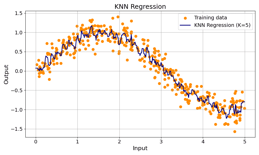
    KNN regression with K equals five predicting a jagged step like curve through noisy sinusoidal training points

    Figure 1: KNN regression (K=5) on a noisy sine wave: each prediction averages the 5 nearest targets, producing a locally-flat, step-like curve that follows the trend but clips the peaks and troughs, the signature of local averaging.

    Mathematical Formulation:
    \hat{y} = \frac{1}{K} \sum_{i=1}^{K} y_i
    \hat{y}(x_q) = \frac{\sum_{i=1}^{K} w_i \cdot y_i}{\sum_{i=1}^{K} w_i}
    w_i = \frac{1}{d(x_q, x_i) + \epsilon}

    Where:

    • \hat{y} is the prediction for the query point; y_i the target of the i-th nearest neighbor; K the number of neighbors (first formula: uniform average).
    • In the weighted variant, w_i is inversely proportional to the distance d(x_q, x_i) between query and neighbor: closer points influence the prediction more.
    • \epsilon is a small constant avoiding division by zero when a neighbor sits exactly on the query.

    Login to view more content
  • ML0054 KNN Classification

    Please explain how KNN classification works.

    Answer

    K-Nearest Neighbors (KNN) is a simple, non-parametric algorithm that predicts a label by majority vote among the K nearest neighbors of a test point, using a chosen distance metric. It is intuitive and effective for small datasets, though less efficient on large-scale data.

    (1) Instance-Based Method: KNN learns no explicit model; it stores the training data and predicts from similarity.
    (2) Distance-Based Classification: For a test point, it computes the distance to every training point (e.g., Euclidean).
    (3) Majority Vote: It selects the K closest neighbors and assigns the most frequent label among them.
    (4) Sensitive To K And Metric: Performance depends on the choice of K and the distance measure (Euclidean, Manhattan, …).
    (5) No Training Phase: All computation happens at prediction time: hence “lazy learning”.

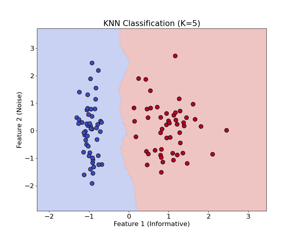
    KNN with K equals five decision regions over two classes where only the horizontal feature is informative

    Figure 1: KNN (K=5) decision regions: the boundary wiggles because each query point polls its 5 nearest neighbors: local votes trace the class structure instead of fitting a global line. Note only Feature 1 is informative here; the vertical wiggle is the noise feature leaking into the vote.

    Mathematical Formulation:
    \mathrm{distance}(x, y) = \sqrt{\sum_{i=1}^{n} (x_i - y_i)^2}
    \hat{y} = \arg\max_{c \in \mathcal{C}} \; \sum_{i=1}^{K} \mathbb{1}(y_i = c)

    Where:

    • x_i and y_i are the i-th features of the query and training points; n is the number of features (first formula: Euclidean distance).
    • \hat{y} is the predicted class for the query point; \mathcal{C} is the set of all classes; K is the number of neighbors polled.
    • y_i is the label of the i-th neighbor and \mathbb{1}(y_i = c) the indicator counting that neighbor’s vote for class c.

    Login to view more content