Interview for Machine Learning

Tag: NN

DL0051 Sparsity in NN
Explain the concept of “Sparsity” in neural networks.
Answer
Sparsity in neural networks refers to the property that many parameters (weights) or activations are exactly zero (or very close to zero).
This leads to lighter, faster, and more interpretable models. Techniques such as L1 regularization, pruning, and ReLU activations help enforce sparsity, making networks more efficient without compromising performance.
Common techniques and their equations:
(1) L1 Regularization (encourages sparse weights)
$L = L_{\text{task}} + \lambda \sum_i |w_i|$
Where:
$w_i$ represents the i-th model weight
$\lambda$ controls the strength of sparsity
(2) ReLU Activation (induces sparse activations)
$\mathrm{ReLU}(x) = \max(0, x)$
Where:
$x$ is the neuron input.
The plot below shows weight distributions trained without using L1 and with L1-induced sparsity.
Login to view more content
December 30, 2025
ML0066 Model Capacity
Without activation functions, how does the model capacity of a 2‑layer neural network compare to a 20‑layer network?
Answer
In the absence of activation functions, a neural network, regardless of depth, is equivalent to a single linear transformation. The model capacity is limited by the expressiveness of linear mappings, with the maximum rank determined by layer widths and thus the parameter count. The network with more parameters, whether 2-layer or 20-layer, can represent a higher-rank transformation, but depth alone provides no additional ability to capture non-linear relationships.
Without activation functions, all layers collapse to a single linear transformation:
$y = W_{\text{eff}} x + b_{\text{eff}}$
Where:
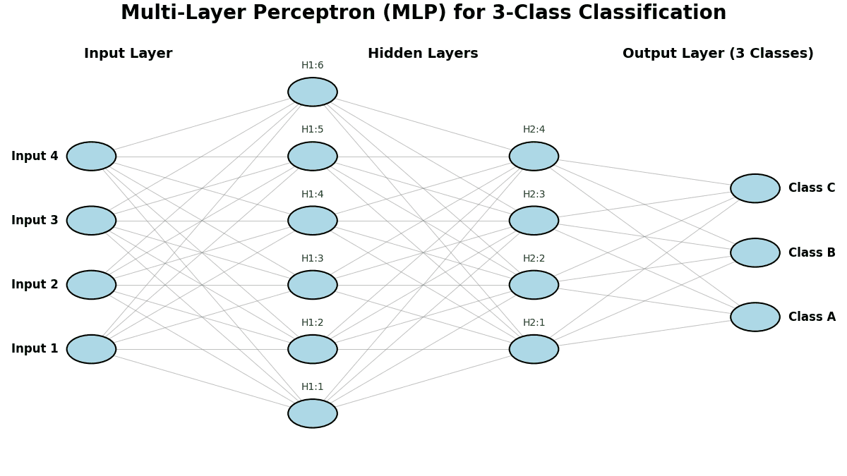
$W_{\text{eff}}$ is the effective weight matrix.
$b_{\text{eff}}$ is the effective bias.
Representational capacity is the same for both 2-layer and 20-layer networks.
Parameter count also depends on the width of layers, not just depth.
Formula for fully connected layers:
$\mbox{Params per layer} = d_\text{in} \times d_\text{out} + d_\text{out}$
Where:
$d_\text{in}$ is the input dimension.
$d_\text{out}$ is the output dimension of that layer.
A wider 2-layer network can have more parameters than a narrow 20-layer network. Conversely, a sufficiently deep 20-layer network can have more parameters than a narrow 2-layer network.
Neither network can model nonlinear data, as shown below.
Login to view more content
August 16, 2025
ML0049 Logistic Regression II
Please compare Logistic Regression and Neural Networks.
Answer
Logistic Regression is a straightforward, linear model suitable for linearly separable data and offers good interpretability. In contrast, Neural Networks are powerful, non-linear models capable of capturing intricate patterns in large datasets, often at the expense of interpretability and higher computational demands.
The table below compares Logistic Regression and Neural Networks in more detail.
Login to view more content
June 10, 2025
DL0019 Go Deep
How does increasing network depth impact the learning process?
Answer
Increasing network depth enhances feature learning and model power, but brings training instability, higher cost, and design complexity.
Increasing network depth can bring benefits:
(1) Improved Feature Hierarchy: Deeper layers can learn more abstract, high-level features. In image classification, early layers learn edges, deeper ones learn shapes and objects.
(2) Increased Model Capacity: More layers allow the network to model more complex functions and patterns.
(3) Improved Efficiency for Complex Functions: For certain complex functions, deep networks can represent them more efficiently with fewer neurons compared to shallow ones.
Increasing network depth can bring challenges:
(1) Vanishing/Exploding Gradients: Gradients can become extremely small or large as they propagate through many layers, hindering effective training, e.g., “Without techniques like skip connections, a 100-layer network might struggle to learn because gradients vanish before reaching early layers.“
(2) Increased Computational Cost (Challenge): Training deeper networks requires significantly more computational resources and time.
(3) Higher Data Requirements (Challenge): Deeper models have more parameters and are more prone to overfitting if not trained on large datasets.
The following example visually compares a shallow and a deep neural network on learning a complex function.
Login to view more content
May 30, 2025
ML0046 Forward Propagation
Please explain the process of Forward Propagation.
Answer
Forward propagation is when a neural network takes an input and generates a prediction. It involves systematically passing the input data through each layer of the network. A weighted sum of the inputs from the previous layer is calculated at each neuron, and then a nonlinear activation function is applied. This process is repeated layer by layer until the data reaches the output layer, where the final prediction is generated.
Here is the process of Forward Propagation:
(1) Input Layer: The network receives the raw input data.
(2) Layer-wise Processing:
Linear Combination: Each neuron calculates a weighted sum of its inputs and adds a bias.
Non-linear Activation: The resulting value is passed through an activation function (e.g., ReLU, sigmoid, tanh) to introduce non-linearity.
(3) Propagation Through Layers: The output from one layer becomes the input for the next layer, progressing through all hidden layers.
(4) Output Generation: The final layer applies a function (like softmax for classification or a linear function for regression) to produce the network’s prediction.
Login to view more content
May 27, 2025
ML0045 Multi-Layer Perceptron
What is a Multi-Layer Perceptron (MLP)? How does it overcome Perceptron limitations?
Answer
A Multi-Layer Perceptron (MLP) is a feedforward neural network with one or more hidden layers between the input and output layers. Hidden layers in MLP use non-linear activation functions (like ReLU, sigmoid, or tanh) to model complex relationships. MLP can be used for classification, regression, and function approximation. MLP is trained using backpropagation, which adjusts the weights to minimize errors.
Overcoming Limitations:
(1) Learn non-linear: Unlike a single-layer perceptron that can only solve linearly separable problems, an MLP can learn non-linear decision boundaries, handling problems such as the XOR problem.
(2) Universal Approximation: With enough neurons and layers, an MLP can approximate any continuous function, making it a powerful model for various applications.
The plot below illustrates an example of a Multi-Layer Perceptron (MLP) applied to a classification problem.
Login to view more content
May 26, 2025
ML0044 Perceptron
Describe the Perceptron and its limitations.
Answer
The perceptron is a simple linear classifier that computes a weighted sum of input features, adds a bias, and applies a step function to produce a binary decision. The perceptron works well only for data sets that are linearly separable, where a straight line (or hyperplane in higher dimensions) can separate the classes.
The perception output can be calculated by
$y = f(w^T x + b)$
Where:
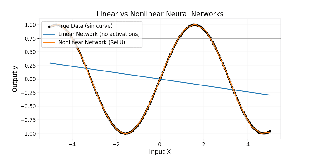
$y$ is the predicted output (0 or 1)
$w$ is the weight vector
$x$ is the input vector
$b$ is the bias term
$f(\cdot)$ is the activation function (typically a step function)
Below shows a perceptron diagram.

Limitations for using perception:
(1) Linearly Separable Data Only: Cannot solve problems like XOR, which are not linearly separable.
(2) Single-Layer Only: Cannot model complex or non-linear patterns.
(3) No Probabilistic Output: Outputs only binary values, not confidence or probabilities.
Login to view more content
May 26, 2025
ML0041 Concept of NN
Please explain the concept of a Neural Network.
Answer
A neural network (NN) is a machine learning model composed of layers of interconnected neurons. It learns patterns in data by adjusting weights through training, enabling it to perform tasks like classification, regression, and more.
(1) Inspired by Biology: Neural networks are computer systems modeled after the human brain’s network of neurons.
(2) Layered Structure: Neural networks consist of an input layer, one or more hidden layers, and an output layer.
(3) Neurons and Activation: Each neuron performs a weighted sum of its inputs, adds a bias, and applies an activation function to produce an output. Weights and Biases are learnable parameters adjusted during training. Activation Functions can introduce non-linearity (e.g., ReLU, Sigmoid).
(4) Learning Process: Neural networks learn by adjusting the weights and biases through training algorithms such as backpropagation, minimizing errors between predictions and actual results.
(5) Versatility in Applications: Neural networks can identify complex patterns, making them suitable for tasks like image recognition, natural language processing, and data classification.
Below shows an example of an NN.
Login to view more content
May 24, 2025
ML0037 Bias in NN
Why is bias used in neural networks?
Answer
Bias in Neural Networks is used to introduce flexibility and adaptability in learning.
(1) Shifts Activation Threshold: Allows a neuron’s activation function to move left or right, so it can fire even when inputs sum to zero.
(2) Avoids Origin Constraint: Lets decision boundaries and fitted functions not be forced through the origin (0,0).
(3) Increases Flexibility: Provides an extra learnable parameter for better approximation of complex functions.
(4) Compensates for Imbalance: Helps adjust for biases in data or features.
Login to view more content
May 17, 2025
DL0012 Zero Padding
Why is zero padding used in deep learning?
Answer
Zero padding in deep learning, particularly in CNNs, is a technique of adding layers of zeros around the input to convolutional layers. This is crucial for maintaining the spatial dimensions of feature maps, preventing loss of information at the image or feature map borders, enabling the use of larger receptive fields via larger kernels, and providing control over the output size of convolutional operations. Ultimately, it helps in building deeper and more effective neural networks by preserving important spatial information throughout the network.
Here are the benefits of using zero padding for CNN.
(1) Preserves Spatial Dimensions: Prevents feature maps from shrinking after convolution.
Below is a 2D image example for using zero padding in CNN.

(2) Retains Boundary Information: Ensures edge pixels are processed adequately.
(3) Enables Larger Kernels: Allows using bigger filters without excessive size reduction.
(4) Controls Output Size: Provides a mechanism to manage the dimensions of output feature maps.
Beyond CNNs, zero padding plays a vital role in deep learning by standardizing variable-length sequences in tasks like NLP and time-series modeling. It ensures inputs have uniform dimensions for efficient batching and computation, enhances frequency resolution in spectral analyses, and allows for effective loss masking to focus learning on actual data.
(1) Standardizing Variable-Length Inputs: In NLP and time-series analysis, zero padding ensures that sequences of varying lengths have a uniform size. This uniformity is crucial for batch processing and for models like recurrent neural networks (RNNs) or transformers.
(2) Attention Masking in Transformers: Padding tokens in Transformer inputs are assigned zero values and then excluded via padding masks in self-attention layers, preventing the model from attending to irrelevant positions in the sequence.
Login to view more content
May 11, 2025