Interview for Machine Learning

Tag: NN

ML0034 Backpropagation
What is backpropagation?
Answer
Backpropagation, backward propagation of errors, is the central algorithm by which multilayer neural networks learn. At its core, it efficiently computes how each weight and bias in the network contributes to the overall prediction error (loss). Then, it updates those parameters in the direction that reduces the error the most.
By combining the chain rule from calculus with gradient‑based optimization (e.g., gradient descent), backpropagation makes training deep architectures tractable and underpins virtually all modern advances in deep learning.
Steps to conduct Backpropagation:
(1) Forward Pass: Inputs are propagated through the network to compute outputs. Intermediate activations are stored for later use.
(2) Compute Loss: Use a loss function to compare the network’s output to the actual target values.
(3) Backward Pass (Error Propagation): The error is computed at the output layer. The chain rule is applied to recursively calculate the gradients of the loss for each weight, starting from the output layer back to the input layer.
(4) Gradient Calculation: For every neuron, determine how much its weights contributed to the error by computing partial derivatives.
(5) Update Weights: Adjust the weights using an optimization algorithm (e.g., gradient descent), by subtracting a fraction (learning rate) of the computed gradients. This step is repeated iteratively to gradually minimize the loss.
More details for step (3): Backward Pass (Error Propagation)
At the Output Layer:
Imagine a neuron with an output value $a$ (its activation) and a weighted sum $z$ computed as:
$\mbox z = w_1 x_1 + w_2 x_2 + \dots + w_n x_n + b$
Suppose we use the mean squared error (MSE) as our loss function:
$\mbox L = \frac{1}{2} (T - a)^2$
Where $T$ is the target value.
The derivative of the loss to the activation is:
$\frac{dL}{da} = a - T$
To update weights, we need to know how the loss changes to $z$ . Using the chain rule, we have:
$\frac{dL}{dz} = \frac{dL}{da} \cdot \frac{da}{dz}$
For example, if the activation function is sigmoid, then:
$\frac{da}{dz} = a (1 - a)$
For Hidden Layers:
Consider a hidden neuron $j$ that feeds into the output neurons. Its contribution to the loss is influenced by all neurons it connects to in the subsequent layer. The backpropagated error for neuron $j$ is given by:
$\frac{dL}{dz_j} = \left( \sum_{k} \frac{dL}{dz_k} \cdot w_{jk} \right) \cdot f'(z_j)$
Here, $f'(z_j)$ is the derivative of the activation function at neuron $j$ .
More details for step (4): Gradient Calculation
For Each Weight:
Once you have the error signal $\frac{dL}{dz}$ for a neuron, the gradient with respect to a weight $w_i$ connected to input $x_i$ is:
$\frac{dL}{dw_i} = \frac{dL}{dz} \cdot x_i$
This shows that the gradient is directly proportional to the input, linking how much weight its contribution had on the final error.
For the Bias:
Since the bias b contributes to $z$ with a derivative of 1, the gradient for the bias is simply:
$\frac{dL}{db} = \frac{dL}{dz}$
Login to view more content
May 8, 2025
ML0033 All Zeros Init
How does initializing all weights and biases to zero affect a neural network’s training?
Answer
Initializing all weights and biases to zero forces neurons to behave identically, leading to uniform gradient updates that prevent the network from learning diverse representations.
(1) Symmetry Problem: Neurons receive identical gradients, causing them to learn the same features rather than developing distinct representations.
(2) Limited Representational Capacity: The network cannot capture complex, varied patterns because all neurons behave identically.
(3) Slow/No Convergence: The lack of Representational Capacity further makes it difficult for the model to update to the optimal weights.
(4) Zero Output (Potentially): For some activation functions (like ReLu), with zero weights and biases, the initial output of every neuron will be zero. This can lead to zero gradients in the subsequent layers, halting the learning process entirely.
Here is an example comparing initializing all weights and biases to zero vs random initialization for a binary classification problem.
Login to view more content
May 6, 2025
DL0011 Fully Connected Layer
Can you explain what a fully connected layer is？
Answer
A Fully Connected (FC) Layer, or Dense Layer, is one where every neuron connects to all neurons in the previous layer. It computes a weighted sum of inputs, adds a bias, and applies an activation function to introduce non-linearity. This allows the network to learn complex feature combinations.
FC layers learn complex combinations of features but can be parameter-heavy and lose spatial context while flattening the feature maps.
Global Average Pooling (GAP) summarizes each feature map into a single value, reducing dimensionality and improving spatial robustness with no added parameters.
GAP followed by a small FC layer, is often used to replace the flatten operation with a large FC layer at the end of Convolutional Neural Networks (CNNs) for classification tasks.
The image below shows examples of parameter comparisons between using Flatten + FC and GAP + FC. There is a total of 6 classes and 8 channels.
Login to view more content
May 3, 2025
DL0010 Receptive Field
What is the receptive field in convolutional neural networks, and how do you calculate it?
Answer
In convolutional neural networks (CNNs), the receptive field of a neuron is the region of the input image that can affect that neuron’s activation. Receptive field Increases in deeper layers, allowing the network to learn hierarchical features.
Use the following iterative formula to calculate the Receptive field:
$RF_l = RF_{l-1} + (k_l - 1) \times \prod_{i=1}^{l-1} s_i$
Where:
$RF_l$ represents the receptive field size in layer $l$ . $RF_0 = 1$ for the input layer.
$k_l$ represents the kernel size of layer $l$ .
$s_i$ represents the stride of layer $i$ .
The following image shows an example of receptive field size growth in a CNN.
K means kernel size, S means stride, and D means dilation rate.
Login to view more content
May 1, 2025
DL0004 Small Kernels
What are the key advantages of using small convolutional kernels, such as 3×3, over utilizing a few larger kernels in deep learning architectures?
Answer
Using small convolutional kernels instead of a few larger kernels offers several significant advantages in deep learning architectures:
(1) Deeper Networks & More Non-Linearity: Stacking multiple 3×3 layers (e.g., three 3×3 layers) allows for a deeper network with more non-linear activation functions compared to a single large kernel.
(2) Reduced Parameters: Multiple small kernels can achieve the same receptive field as a larger one, but with fewer parameters.
Example: Two stacked 3×3 layers ( $18 \cdot C_{in} \cdot C_{out}$ total parameters) have the same receptive field as a 5×5 layer ( $25 \cdot C_{in} \cdot C_{out}$ total parameters) but fewer parameters.

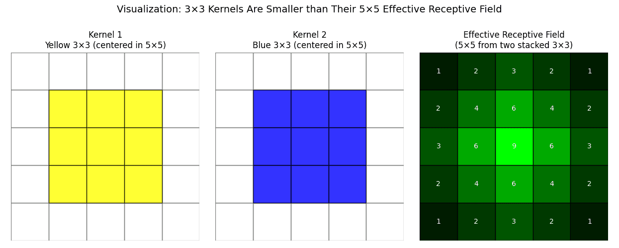
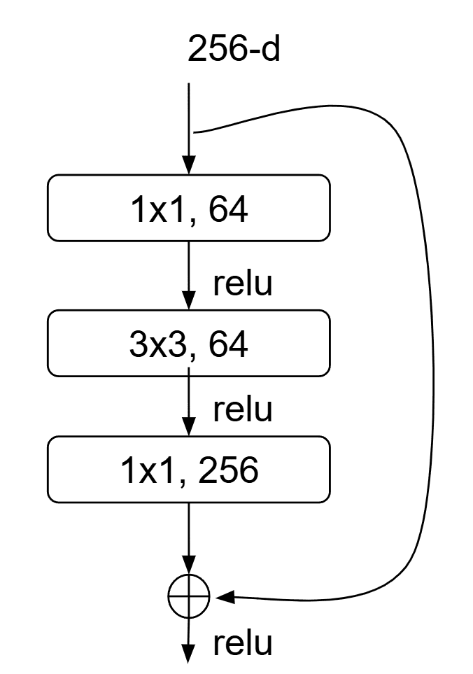
(3) Computational Efficiency: Fewer parameters in smaller kernels generally lead to lower computation costs during training and inference.
(4) Gradual Receptive Field Expansion: Successive 3×3 convolutions progressively build a larger receptive field while maintaining fine detail. (3×3 filters focus on local detail capture with pixel neighborhoods, ideal for textures or edges.)
Login to view more content
April 29, 2025
DL0003 1×1 Convolution
What are the benefits of using 1×1 convolutional layers in deep learning architectures?
Answer
A 1×1 convolution, also known as a pointwise convolution, is a convolutional operation where the kernel size is 1×1, which plays several crucial roles in deep learning architectures.
(1) Dimensionality control: 1×1 convolution can reduce or expand the number of feature maps, trading off representational capacity and computational cost.
For example, Bottleneck designs: In architectures like ResNet’s bottleneck block, a 1×1 conv first reduces channels (e.g., 256→64), then a 3×3 conv processes those, and finally another 1×1 conv expands back (64→256) to restore capacity while keeping compute manageable.
(2) Increased Network Depth with Controlled Cost: Allows for the design of deeper networks by reducing channel dimensionality before computationally expensive spatial convolutions.
(3) Cross-Channel Feature Fusion: Enables interaction and combination of information across different feature channels at the same spatial location.
(4) Non-linear mixing: When followed by activations (ReLU, etc.), 1×1 convolutions introduce non‐linear channel mixing that enhances model expressiveness.
Login to view more content
April 29, 2025
DL0002 All Ones Init
What are the potential consequences of initializing all weights to one in a deep learning model?
Answer
Below are the key consequences of initializing all weights in a deep-learning model to one (a constant non-zero value), illustrating why random, scaled initializations (e.g., Xavier/He) are essential.
(1) Symmetry Problem: Neurons receive identical gradients, causing them to learn the same features rather than developing distinct representations.
(2) Limited Representational Capacity: The network cannot capture complex, varied patterns because all neurons behave identically.
(3) Slow/No Convergence: The lack of Representational Capacity further makes it difficult for the model to update to the optimal weights. (The below image shows an example for training loss comparison for ones initialization vs random initialization)

(4) Activation Saturation: Can push neurons into saturated regions of activation functions (e.g., sigmoid, tanh), leading to vanishing gradients.
Login to view more content
April 28, 2025
DL0001 Residual Connection
Why are residual connections important in deep neural networks?
Answer
Residual connections, also known as skip connections, are vital in deep neural networks primarily because they tackle the infamous vanishing gradient problem and help with the related issue of network degradation as the network depth increases.
Residual connection is often expressed by the following equation:
$y = F(x) + x$
Where:
$F(x)$ represents the residual mapping that the network learns (i.e., what needs to be added to the input $x$ to achieve the desired output).
$x$ is the input to the residual block.
(1) Tackle vanishing gradient problem:
Residual connections create a direct shortcut for gradient flow by incorporating an identity mapping into the learned transformation. This ensures that even if the gradient through the learned component is small, a strong, direct gradient component persists, preventing vanishing gradients in deep networks. This improves gradient flow during backpropagation, reducing vanishing gradients and enabling the training of very deep networks.
(2) Address network degradation:
Residual connections mitigate the degradation problem often seen in deep networks. Without these connections, simply stacking more layers can result in higher training errors, as the network struggles to update its weights effectively. With residual connections, any layer that doesn’t contribute useful information can effectively learn to output zeros in the residual branch, letting the network default to an identity mapping.
Login to view more content
April 23, 2025
ML0007 Dropout
What is dropout in neural network training?
Answer
Dropout is a regularization technique used during neural network training to prevent overfitting.
During each training step, a fraction of the neurons (and their corresponding connections) are randomly “dropped out” (i.e., set their activations to zero). This forces the network to learn more robust features because it can’t rely on any single neuron; instead, it learns distributed representations by effectively training an ensemble of smaller sub-networks. This will improve the model’s ability to generalize to unseen data.
Login to view more content
March 16, 2025