DL0004 Small Kernels

Written by

What are the key advantages of using small convolutional kernels, such as 3×3, over utilizing a few larger kernels in deep learning architectures?

Answer

Using small convolutional kernels instead of a few larger kernels lets a network reach the same receptive field with fewer parameters, more depth, and more non-linearity. A stack of $3\times3$ convolutions matches the spatial coverage of a single large kernel while inserting an activation between each layer, which increases the network’s representational power. This design is the foundation of architectures such as VGG.

(1) Deeper Networks & More Non-Linearity: Stacking multiple $3\times3$ layers (e.g., three of them) creates a deeper network with more non-linear activation functions than a single large kernel.
(2) Reduced Parameters: Multiple small kernels achieve the same receptive field as a larger one with fewer parameters: two stacked $3\times3$ layers use $18\cdot C_{in}\cdot C_{out}$ weights versus $25\cdot C_{in}\cdot C_{out}$ for one $5\times5$ layer.
(3) Computational Efficiency: Fewer parameters generally mean lower FLOPs during training and inference.
(4) Gradual Receptive Field Expansion: Successive $3\times3$ convolutions progressively build a larger receptive field while preserving local detail capture, ideal for textures and edges.

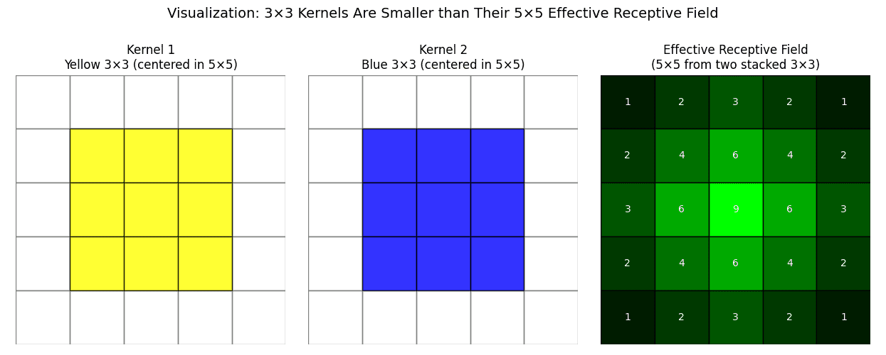
Two stacked 3x3 convolutions viewing the same 5x5 input region as a single 5x5 convolution.

Figure 1: Two stacked $3\times3$ convolutions see the same $5\times5$ input region as one $5\times5$ convolution, but with an extra non-linearity in between.

Kernel Composition: Two stacked $3\times3$ kernels compose into a single equivalent $5\times5$ kernel (their full discrete convolution), which is exactly why the receptive fields match.

Two all-ones 3x3 kernels composing into an equivalent 5x5 kernel with coefficients formed by their full discrete convolution.

Figure 2: Two $3\times3$ kernels compose into one equivalent $5\times5$ kernel; stacking keeps them separate: 18 weights plus an extra non-linearity instead of a 25-weight merge.

Mathematical Formulation:
$P_k = k^2 \cdot C_{in} \cdot C_{out}$
$RF_l = 1 + l\cdot(k-1)$
$2 \times 3^2 = 18 \text{ vs } 5^2 = 25$
$3 \times 3^2 = 27 \text{ vs } 7^2 = 49$

Where:

$P_k$ is the parameter count of one $k\times k$ convolution (ignoring biases).
$C_{in}$ and $C_{out}$ are the input and output channel counts.
$RF_l$ is the receptive field after $l$ stacked layers; two $3\times3$ layers give $RF=5$ , three give $RF=7$ .