
What is LoRA, and can you explain the low-rank decomposition idea and why it is parameter-efficient?
Answer
LoRA (Low-Rank Adaptation) freezes every pretrained weight matrix and learns only a rank-constrained update beside it: instead of training  with a full
 update, it factors the update as
 with
 ,
 and
 . The motivation is the intrinsic-dimension hypothesis: adapting a large pretrained model to a downstream task moves the weights along a very low-dimensional subspace, so a rank-8 or rank-16 correction captures almost all of the useful change. For one
 attention projection, a rank-16 factorization trains 131,072 numbers instead of 16.8M, roughly 0.78% of the matrix. The efficiency that matters in practice is not forward FLOPs, which barely change, but optimizer and gradient state: Adam keeps two moments plus an fp32 master copy per trainable parameter, so shrinking the trainable set by two or three orders of magnitude is what turns a multi-node job into a single-GPU job. At inference the product can be folded back with
 , so a merged LoRA adds zero latency compared with the original model.
(1) Frozen Base, Additive Branch: the pretrained matrix never receives a gradient; all learning happens in the parallel  branch whose output is added to the frozen path.
(2) Rank Is The Budget Knob: parameter count is  and grows linearly in
 , while the full matrix costs
 , so the ratio is tiny for any practical rank.
(3) Zero Initialization On One Factor:  gets a random Gaussian init and
 is initialized to zeros, so
 at step 0 and training starts exactly at the pretrained function.
(4) Memory Savings Come From Optimizer State: gradients and Adam moments exist only for adapter parameters, which is where the 8x reduction in peak training memory comes from, not from cheaper matrix multiplies.
(5) Mergeable And Swappable: a task adapter is a few tens of MB, so many tasks can share one frozen base, either merged per deployment or batched as separate adapters in a single server.
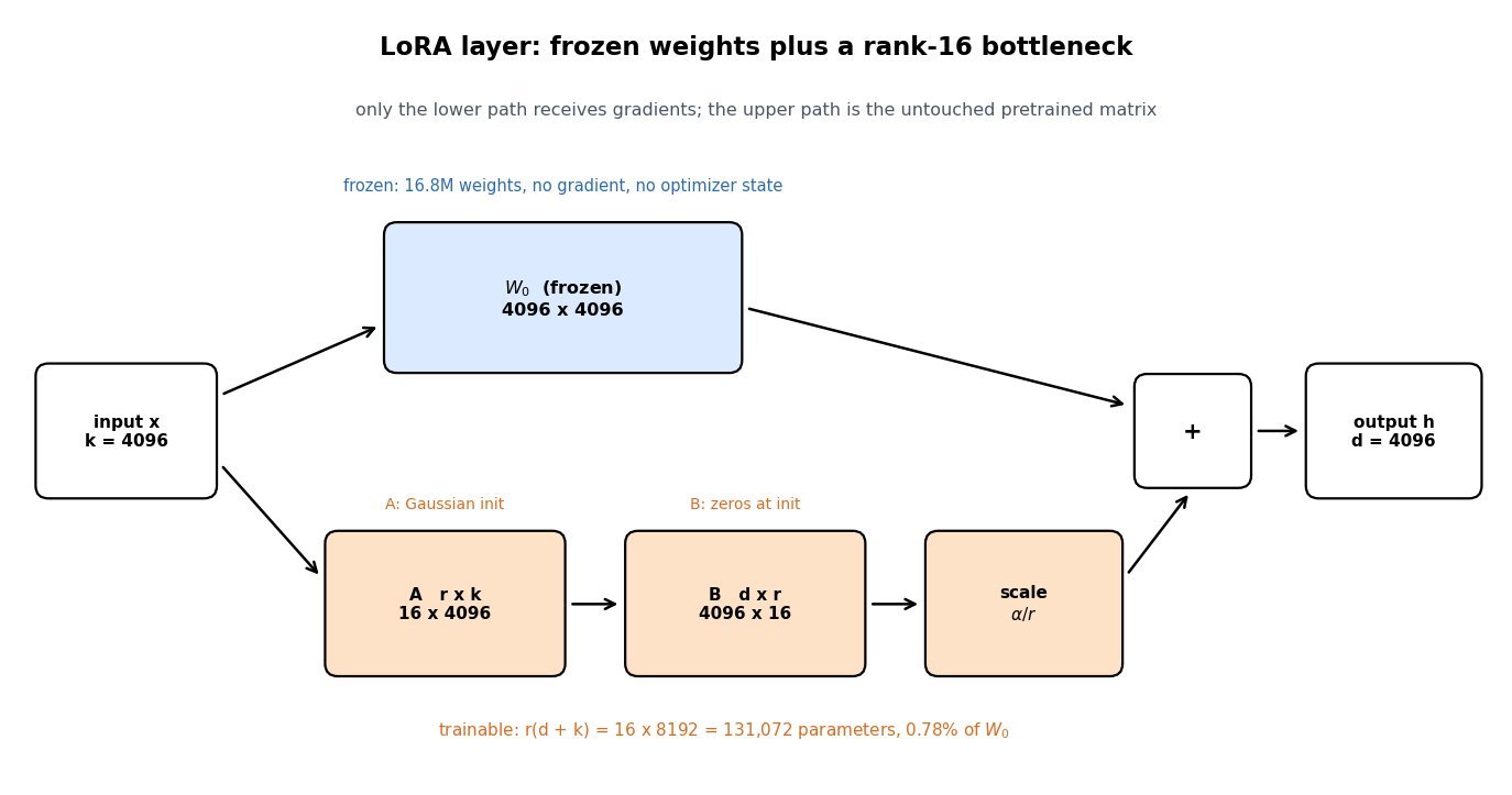
Figure 1: A LoRA layer keeps the frozen 16.8M-parameter projection untouched and routes the input through a rank-16 bottleneck whose 131,072 trainable parameters are added back, scaled by  .
Two implementation details do most of the work. The scaling factor decouples the effective update magnitude from the rank, so raising to add capacity does not silently multiply the learning rate on the adapter branch; the common convention is to fix  and sweep . The choice of target modules matters more than the rank in most experiments: the original paper adapted only the attention query and value projections, while current practice applies LoRA to all linear layers including the MLP, which raises trainable parameters to about 42M on an 8B model but consistently closes the gap to full fine-tuning. One caveat on merging: if the base weights are quantized, folding a bf16 adapter into a 4-bit matrix reintroduces quantization error, so quantized deployments usually keep the adapter separate.
Mathematical Formulation:


Where:
 is the layer output and the input activation for one token.
- is the frozen pretrained matrix, and is the learned correction.
- and are the trainable factors; the rank satisfies , which forces .
- is a fixed scaling constant, so keeps the update magnitude roughly rank-independent.
- is the trainable count per adapted matrix and its fraction of the full matrix; with and this gives 131,072 parameters and .
- Required initial condition: with Gaussian, so before the first step; the last line is the merge applied after training.
 is the layer output and
 the input activation for one token.
 is the frozen pretrained matrix, and
 is the learned correction.
 .
 is the trainable count per adapted matrix and
 its fraction of the full matrix; with
 and
 this gives 131,072 parameters and
 .
 with
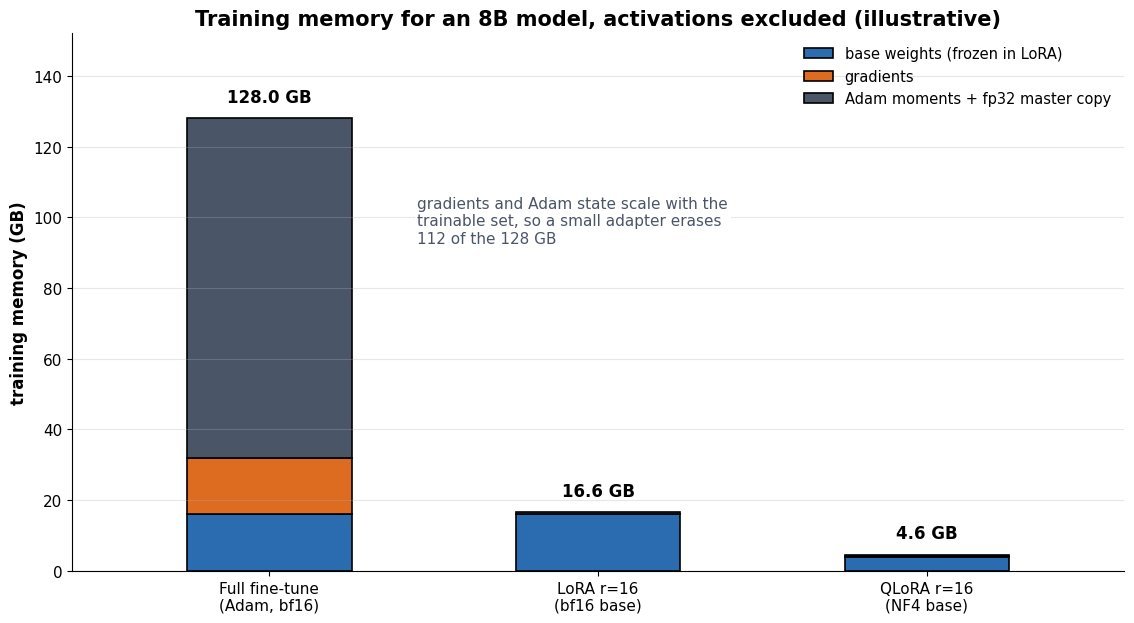
Figure 2: Illustrative training memory for an 8B model before activations: full fine-tuning spends 96 GB on Adam state alone, LoRA with 41.9M trainable parameters needs about 16.6 GB, and a 4-bit frozen base drops that to about 4.6 GB.
| Property | LoRA | Full Fine-Tuning | Bottleneck Adapters |
|---|---|---|---|
| Trainable parameters (8B model) | 41.9M at r=16 on all linear layers, about 0.5% | 8.0B, all of them | Comparable order, set by bottleneck width |
| Added inference latency | None once merged into the base weights | None | Extra sequential layers, noticeable at small batch |
| Peak training memory | About 17 GB, or 5 GB with a 4-bit base | About 128 GB with Adam in mixed precision | Similar to LoRA |
| Multi-task serving | Hundreds of small adapters over one frozen base, batchable | One 16 GB checkpoint per task | Swappable but cannot be merged away |
| Quality ceiling | Matches full tuning on most instruction and style adaptation | Upper bound, clearly better for large domain shift | Roughly on par, less used today |
Leave a Reply