Author: admin

DL0080 Tokenization in LLMs

Explain tokenization in large language models.

Answer

Tokenization is the reversible mapping between raw text and the sequence of integer ids a language model actually consumes, drawn from a fixed vocabulary of size $V$ . Modern LLMs use subword vocabularies that sit between characters (short vocab, very long sequences) and words (huge vocab, unavoidable out-of-vocabulary gaps), and the dominant recipe is byte-level BPE: count adjacent symbol pairs over a training corpus, greedily merge the most frequent pair, and repeat until the vocabulary reaches its target size. Because the base alphabet is the 256 possible bytes rather than Unicode characters, any input is representable and there is no UNK token, at the cost of spending several tokens per character on scripts the merge table never learned. The tokenizer is frozen before pretraining and is effectively part of the architecture: it fixes the embedding matrix and output projection ( $2Vd$ parameters), it decides how many model passes a sentence costs, and it determines whether the model sees 1024 as one symbol or three. Most surprising LLM behaviors around arithmetic, non-English cost, and trailing whitespace trace back to this layer rather than to the transformer itself.

(1) Subword Is A Middle Ground: character-level models keep the vocabulary tiny but inflate sequence length, and attention is $O(N^2)$ in that length; word-level vocabularies need hundreds of thousands of entries and still miss rare words and typos.
(2) How BPE Is Trained And Applied: training produces an ordered merge list; encoding replays those merges greedily on each pretokenized chunk, so segmentation is deterministic and not a search over the best split.
(3) Pretokenization Comes First: in the GPT-style recipe a regex splits text on whitespace, punctuation, and digit groups before BPE runs, which is why the leading space belongs to the token (" the" and "the" are different ids) and why, with standard pretokenization, merges do not cross word boundaries; that constraint comes from the pretokenizer rather than from BPE itself, and implementations that skip or relax it (see SuperBPE below) do learn multi-word tokens.
(4) Vocabulary Size Is A Compute Knob: raising $V$ lowers fertility (tokens per word) so each sentence needs fewer forward passes, but it grows the embedding and softmax cost, which is why the field drifted from 32k to 128k vocabularies (Llama 2 → Llama 3) as models got larger.
(5) The Failure Modes Users Notice: digit grouping degrading arithmetic, non-English prompts costing two to three times more tokens for the same content, glitch tokens whose embeddings were barely trained, and special chat-template ids that must never be injectable from user text.

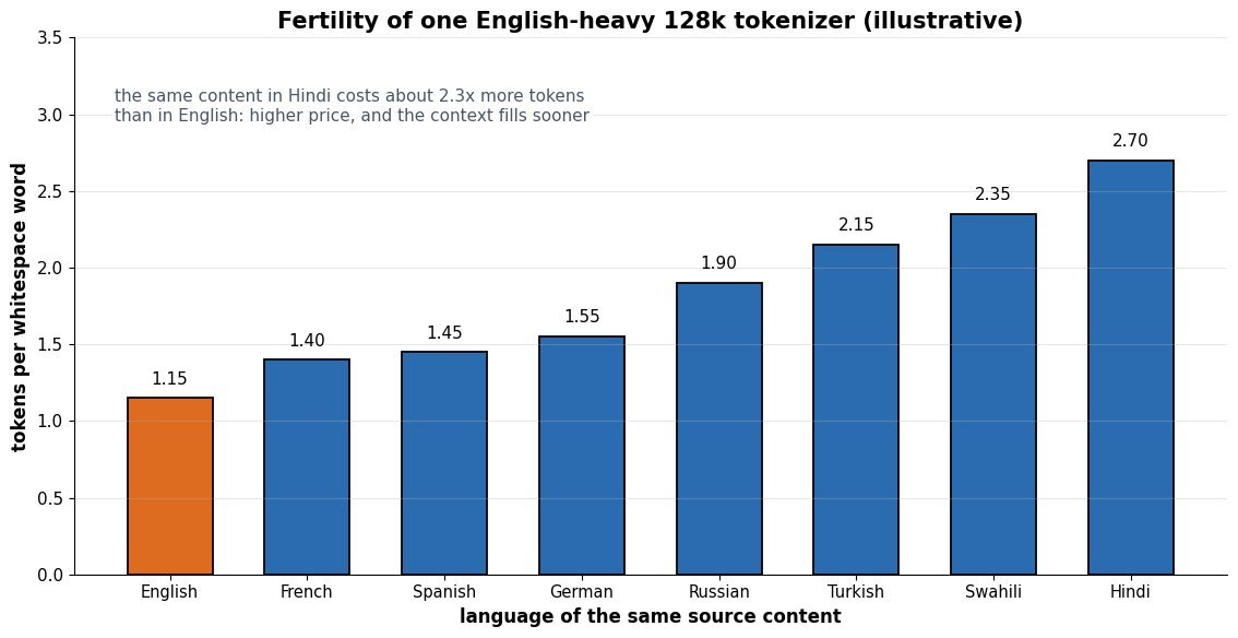
Bar chart of tokens per whitespace word for eight languages under one English-heavy tokenizer: English 1.15, French 1.40, Spanish 1.45, German 1.55, Russian 1.90, Turkish 2.15, Swahili 2.35, Hindi 2.70

Figure 1: Illustrative fertility gap: with a merge table dominated by English text, the same content in Hindi consumes roughly $2.3\times$ more tokens, so it costs more per request and reaches the context limit sooner.

Two implementation details matter more in production than the choice of merge algorithm. First, digit handling: tokenizers that merge arbitrary digit runs give the model inconsistent units for numbers, so 2024, 202, and 24 share no stable structure and column-wise arithmetic has to be learned per token; Llama 3 and several recent tokenizers instead force digits into groups of at most three, and some research tokenizers split every digit. Second, special tokens such as beginning-of-text and end-of-turn markers are inserted out of band by the chat template, not produced by BPE over user text; if a serving layer lets a user string encode into those ids, the model’s turn structure can be rewritten from inside a prompt. Related traps include unnormalized Unicode (NFC versus NFKC changes ids for accented text), tokenizer and checkpoint version skew, which silently shifts every embedding lookup, and untrained vocabulary rows that surface as glitch tokens the model cannot repeat back.

Mathematical Formulation:
$(a,b)^{*} = \arg\max_{(a,b)} c(a,b)$
$F = \frac{T}{W}$
$P_{\text{emb}} = 2 V d$
$C_{\text{word}} = F \cdot (C_{\text{body}} + 2 V d)$

Where:

$(a,b)^{*}$ is the pair chosen at each BPE training step, and $c(a,b)$ is its frequency as adjacent symbols in the corpus; the merge is appended to an ordered list that encoding later replays.
$F$ is fertility: $T$ tokens produced for $W$ whitespace words, measured per language and per corpus, so it is a property of the tokenizer and the text, not of the model.
$P_{\text{emb}}$ counts the input embedding plus the untied output projection for vocabulary $V$ and hidden width $d$ ; tying the two halves this term but couples input and output geometry.
$C_{\text{word}}$ is the compute per word of text, where $C_{\text{body}}$ is the per-token cost of everything except the vocabulary layers; the two $V$ -dependent effects pull in opposite directions, which is why an interior optimum in $V$ exists and grows with model size.

Two panels versus vocabulary size on a log axis: left panel shows tokens per word falling from about 1.72 at 4k vocab to 1.27 at 512k with diminishing returns, right panel shows relative compute per word dipping to a minimum near 33k vocabulary and rising to about 1.65 at 512k

Figure 2: Illustrative trade-off for a 1B-scale model with $d = 1024$ : shorter sequences from a larger vocabulary stop paying for themselves once the $2Vd$ output-layer cost rivals the transformer body, and the minimum shifts right as $d$ and depth grow.

Feature	Byte-level BPE	WordPiece	Unigram LM
How the vocab is learned	Greedily merge the most frequent adjacent pair, recording an ordered merge list	Merge the pair that most increases corpus likelihood under a unigram model	Start from a large candidate set and prune the tokens whose removal costs the least likelihood (EM)
How text is segmented	Replay merges in training order; deterministic and fast	Longest-match-first greedy scan, with `##` marking continuations	Viterbi search for the most probable segmentation, and it can sample splits for subword regularization
Unseen input	No UNK is possible; the 256-byte alphabet covers all of Unicode	Emits UNK for characters outside the alphabet unless byte fallback is added	Byte fallback is optional in SentencePiece and usually enabled
Where you see it	GPT-2 onward, Llama, Mistral, Qwen	BERT and the encoder family that followed it	T5, ALBERT, and many multilingual encoders

August 15, 2026

DL0079 Scaling Laws Size vs Data

How do scaling laws relate model size to training data requirements?

Answer

Neural scaling laws say that test loss falls as a power law in both parameter count $N$ and training tokens $D$ , plus an irreducible floor, so the two are not independent knobs: a fixed compute budget $C \approx 6ND$ forces a trade between them. Kaplan et al. (2020) fit the loss surface and concluded that most extra compute should go into parameters, which is why GPT-3 used 175B parameters on only about 300B tokens (roughly 1.7 tokens per parameter). Hoffmann et al. (2022, “Chinchilla”) re-ran the sweep with properly decayed learning-rate schedules over more than 400 runs and found the compute-optimal frontier scales both quantities at roughly the same rate, $N_{opt} \propto C^{0.5}$ and $D_{opt} \propto C^{0.5}$ , giving the well-known heuristic of about 20 tokens per parameter. Under that law a 70B model trained on 1.4T tokens beat a 280B model trained on 300B tokens at equal compute. The practical answer to the interview question is therefore: data requirements grow roughly linearly with model size along the compute-optimal frontier, and any deviation from that ratio should be justified by a constraint the loss law does not model, such as a finite corpus or the cost of serving.

(1) Joint Power Law: loss decomposes into an entropy floor plus one shrinking term per resource, $L = E + AN^{-\alpha} + BD^{-\beta}$ , so starving either resource leaves its term dominant and no amount of the other resource can fix it.
(2) Compute Couples The Two: with $C \approx 6ND$ FLOPs (2 for the forward pass and 4 for the backward pass per parameter per token), choosing $N$ fixes $D$ , which is why the question is always “what split”, never “how big”.
(3) IsoFLOP Minima Define The Frontier: sweeping $N$ at fixed $C$ traces a shallow U-shaped curve; the locus of minima across budgets is the compute-optimal frontier, and its slope in log-log space is the exponent you actually care about.
(4) Kaplan Versus Chinchilla: the earlier exponents ( $N_{opt} \propto C^{0.73}$ ) came from a fixed-length cosine schedule truncated early and from parameter counts that excluded embeddings, both of which penalize the long-token runs and bias the fit toward oversized models.
(5) Optimal Does Not Mean Correct: the law optimizes training loss per training FLOP; it says nothing about inference cost, so serving-heavy models are deliberately overtrained far past 20 tokens per parameter.

The empirical procedure behind these numbers is worth stating precisely, because interviewers probe it. You pick a grid of compute budgets, and for each budget you train several models of different widths and depths, always to the token count that exhausts exactly that budget, with the learning rate decayed to its minimum at the end of each run. Plotting final loss against $N$ for one budget yields an IsoFLOP curve whose minimum is flat enough that a factor of two in parameter count often costs under 1% in loss, which is exactly the slack engineers exploit when memory or latency constraints bite.

Four U-shaped IsoFLOP curves of loss versus parameter count on a log x-axis for compute budgets of 1e19, 1e20, 1e21 and 1e22 FLOPs, with minima marked and joined by a dashed frontier line moving right and down

Figure 1: Illustrative IsoFLOP curves from $L = E + AN^{-0.34} + BD^{-0.34}$ with $C = 6ND$ . Each budget’s minimum sits at $D/N \approx 20$ , moving from 0.29B parameters / 5.8B tokens at $10^{19}$ FLOPs to 9.1B parameters / 183B tokens at $10^{22}$ FLOPs, and the basins are shallow near the optimum.

Mathematical Formulation:
$L(N,D) = E + A N^{-\alpha} + B D^{-\beta}$
$C \approx 6ND$
$N_{opt} \propto C^{a}$
$D_{opt} \propto C^{b}$
$a = \frac{\beta}{\alpha + \beta}$
$b = \frac{\alpha}{\alpha + \beta}$
$D_{opt} / N_{opt} \approx 20$

Where:

$L(N,D)$ is expected test loss in nats per token, and $E$ is the irreducible term: the entropy of the data plus whatever the architecture can never represent, so no scaling drives loss to zero.
$N$ is the number of trainable parameters (embeddings included, which is where the Kaplan fit differed) and $D$ is the number of training tokens.
$A, B$ are fitted scale constants and $\alpha, \beta$ are the power-law exponents; Chinchilla’s fit put both near $0.3$ , meaning the two resources have comparable marginal value.
$C$ is training compute in FLOPs; the factor 6 comes from roughly 2 FLOPs per parameter per token forward and 4 backward, and it ignores attention’s quadratic term, which is minor while $d_{model}$ dominates sequence length.
$a, b$ are the frontier exponents obtained by minimizing $L$ subject to the compute constraint; $a + b = 1$ always holds, so if parameters take a larger share of compute growth, tokens must take a smaller one.
The ratio $D_{opt}/N_{opt}$ is constant only when $\alpha = \beta$ ; the “20 tokens per parameter” rule is that special case, and it drifts slowly with budget under asymmetric fits.

Log-log plot of compute-optimal parameter count and token count versus training compute from 1e19 to 1e25 FLOPs, with Chinchilla curves scaling as C to the 0.5 for both quantities and Kaplan curves scaling as C to the 0.73 for parameters and C to the 0.27 for tokens, diverging by more than an order of magnitude at high compute

Figure 2: Illustrative comparison of the two prescriptions, normalized to agree at $10^{19}$ FLOPs. Because the exponents differ ( $0.5$ versus $0.73$ ), the gap compounds: at $10^{24}$ FLOPs one recipe asks for 91B parameters on 1.8T tokens and the other for 1.3T parameters on 130B tokens, about a $14\times$ disagreement in both directions.

Modern frontier practice has moved past the compute-optimal point on purpose. If a model will serve billions of tokens, total lifetime FLOPs are dominated by inference, and a smaller model trained on far more data is cheaper end to end even though its training run is nominally suboptimal. Meta’s Llama 3 8B was trained on roughly 15T tokens, near 1,875 tokens per parameter, almost two orders of magnitude past the Chinchilla ratio, and the authors report the loss was still improving log-linearly at that point. The scaling law is still doing the work here; the objective being minimized has simply changed from training loss per training FLOP to quality per unit of deployment cost.

Regime	Tokens Per Parameter	What It Optimizes	When It Is The Right Call
Kaplan-style (parameter-heavy)	About 1 to 2	Loss under a truncated schedule and an embedding-free parameter count	Essentially never today; understand it to explain why GPT-3 looked the way it did
Chinchilla-optimal	About 20	Best loss for a fixed training budget	Research runs, ablations, and any model whose main cost is the training job
Deliberately overtrained	150 to 2,000 or more	Quality per unit of training plus inference cost	High-traffic serving, on-device targets, fixed memory or latency budgets
Data-constrained	Set by the corpus, not by compute	Loss given a finite unique-token pool with repeated epochs	Specialist domains (code, medical, low-resource languages) where fresh tokens run out

August 15, 2026

DL0078 LLM Training Stages

What are the standard stages of LLM training?

Answer

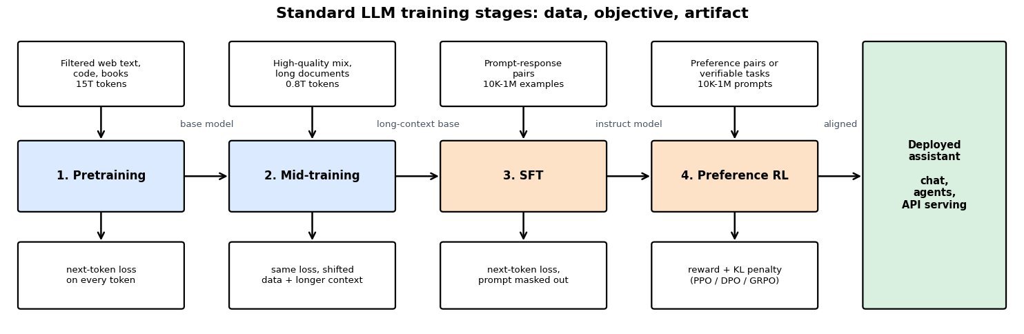
A modern LLM is built in a sequence of stages that share one architecture but differ in data, objective, and scale: pretraining on a web-scale corpus with next-token prediction, an increasingly explicit mid-training phase that reweights the data mix and extends the context window, supervised fine-tuning (SFT) on curated prompt-response pairs, and preference optimization that turns human or programmatic judgments into a training signal (reward model plus PPO, DPO, or reinforcement learning with verifiable rewards). The split is not cosmetic: pretraining consumes well over 90% of the total tokens and FLOPs and is where almost all knowledge and reasoning capacity is acquired, while post-training uses a tiny fraction of the compute to select and expose behaviors the base model already has. Each stage produces a named artifact that the next stage consumes, so the usual lineage is base model → long-context base → instruct model → aligned model. Practical pipelines also interleave evaluation, safety filtering, distillation, and quantization, but those are packaging steps rather than new learning objectives.

(1) Pretraining: self-supervised next-token loss on trillions of filtered web, code, and book tokens, run once at enormous cost; this stage fixes the tokenizer, the parameter count, and the knowledge cutoff.
(2) Mid-Training: continued pretraining on a higher-quality mix with upsampled math, code, and long documents, plus context-length extension and learning-rate annealing, using roughly 1-10% of the pretraining tokens.
(3) Supervised Fine-Tuning: the same cross-entropy loss but computed only on response tokens with the prompt masked out, teaching format, instruction following, and tool-call syntax from $10^4$ to $10^6$ curated examples.
(4) Preference Optimization: optimizes a reward (learned from pairwise comparisons, or computed by a verifier) under a KL penalty toward the SFT reference policy, which is what shifts a model from plausible to preferred.
(5) Compute Asymmetry: post-training is cheap, so it is where iteration happens; anything that requires new knowledge or a longer context has to go back to a pretraining-style stage.

Four-stage LLM training pipeline: filtered web text feeds pretraining with a next-token loss producing a base model, a high-quality long-document mix feeds mid-training producing a long-context base, prompt-response pairs feed SFT with the prompt masked producing an instruct model, and preference pairs or verifiable tasks feed preference RL with a reward plus KL penalty, yielding a deployed assistant

Figure 1: The four canonical stages with their input data, objective, and output artifact. Only the data distribution and loss mask change between stages 1 to 3; stage 4 replaces likelihood with a reward under a KL constraint.

Mathematical Formulation:
$\mathcal{L}_{\mathrm{PT}}(\theta) = -\sum_{t=1}^{T} \log p_{\theta}(x_t \mid x_{1:t-1})$
$\mathcal{L}_{\mathrm{SFT}}(\theta) = -\sum_{t \in \mathcal{A}} \log p_{\theta}(y_t \mid x, y_{1:t-1})$
$\mathcal{L}_{\mathrm{RM}}(\phi) = -\log \sigma\big(r_{\phi}(x,y_w) - r_{\phi}(x,y_l)\big)$
$J(\theta) = \mathbb{E}\big[r_{\phi}(x,y)\big] - \beta\,\mathrm{KL}(\pi_{\theta}\,\|\,\pi_{\mathrm{ref}})$

Where:

$x_{1:t-1}$ is the preceding context and $x_t$ the target token, so pretraining averages this loss over every position of every document.
$x$ is the prompt, $y$ the response, and $\mathcal{A}$ the set of assistant token positions; positions outside $\mathcal{A}$ are masked, which is the only structural difference between SFT and pretraining.
$y_w$ and $y_l$ are the preferred and rejected responses for the same prompt, $r_{\phi}$ is the reward model, and $\sigma$ is the logistic function, giving the Bradley-Terry pairwise objective.
$\pi_{\theta}$ is the policy being trained and $\pi_{\mathrm{ref}}$ the frozen SFT checkpoint; the KL term is what keeps generations fluent instead of collapsing onto reward-model artifacts.
$\beta > 0$ sets the strength of that anchor: small $\beta$ permits reward hacking, large $\beta$ leaves the model barely changed from SFT.

Log-scale bar chart of training tokens per stage: pretraining 15 trillion tokens at 94.9 percent, mid-training 0.8 trillion at 5.1 percent, SFT 0.2 billion at 0.001 percent, and preference RL 4 billion at 0.03 percent

Figure 2: Illustrative token budget for a frontier-scale run. Pretraining and mid-training together see about 99.97% of all tokens, so post-training cannot add missing knowledge, only elicit and shape what is already in the weights.

Post-Training Option	Reward Model + PPO	DPO	Verifiable Rewards (GRPO)
Signal required	Pairwise human preferences, then a learned scalar reward	Pairwise preferences used directly, no reward model	A programmatic checker: unit tests, math answer match, schema validity
Models held in memory	Four: policy, reference, reward, critic	Two: policy and frozen reference	Two plus a sampler: no critic, group baseline replaces it
Online generation	Yes, rollouts dominate wall-clock time	No, offline on a fixed pair dataset	Yes, several samples per prompt
Main failure mode	Reward hacking and length inflation once the reward model is over-optimized	Off-policy drift: pairs stop reflecting the current policy, likelihood of both responses can fall	Only works where correctness is checkable; gaming the checker instead of the task
Typical use	Broad helpfulness and safety at frontier labs with annotation pipelines	Small teams, quick style and tone alignment on limited GPUs	Math, code, and reasoning models where long chains of thought pay off

August 15, 2026

DL0077 LLM Prediction Objective

What is a large language model, and what is its prediction objective?

Answer

A large language model (LLM) is a neural network, in practice a decoder-only Transformer with billions of parameters, trained on trillions of tokens of text to model the probability distribution over token sequences. Its prediction objective is next-token prediction: factor the sequence probability with the chain rule and maximize the log-likelihood of each observed token given its left context, which is identical to minimizing cross-entropy over the vocabulary at every position. The training signal is self-supervised, since the label at position $t$ is simply the token at position $t+1$ , so no human annotation is required and one sequence of length $T$ yields $T-1$ supervised examples in a single forward pass, or a full $T$ when a leading BOS token supplies the context for the first real token. Everything an LLM appears to know (syntax, factual associations, translation, arithmetic, code structure) is a byproduct of driving that one loss down, because accurately predicting the next token over a broad corpus requires modeling the processes that generated the text. Base pretraining optimizes likelihood only; instruction following and refusal behavior come later, from supervised fine-tuning and preference optimization, which change the objective rather than the architecture.

(1) What Makes It “Large”: parameter count in the billions, a training corpus in the trillions of tokens, and a compute budget allocated according to scaling laws, so capability improvements are largely predictable from loss curves rather than architectural novelty.
(2) The Objective Is Autoregressive: the chain-rule factorization plus a causal mask means position $t$ may only attend to positions $1$ through $t$ , which is what makes single-pass training and left-to-right generation consistent with each other.
(3) Loss Is Cross-Entropy Over the Vocabulary: the final layer projects the hidden state to $V$ logits, softmax turns them into a distribution, and the loss is the negative log-probability of the single correct token.
(4) Perplexity Is the Reported Metric: $\mathrm{PPL} = \exp(\mathcal{L})$ is the effective branching factor, so a mean loss of $2.3$ nats means the model is about as uncertain as choosing uniformly among 10 tokens; perplexity depends on the tokenizer and is not comparable across different vocabularies.
(5) Likelihood Is Not Helpfulness: maximizing the likelihood of scraped text also rewards reproducing its errors and its style, and teacher forcing never trains the model to recover from its own mistakes, which is the origin of exposure bias.

Bar chart of a next-token distribution after the prefix The capital of France is: Paris receives 0.83, the receives 0.04, a receives 0.021, now 0.015, located 0.012, and the remaining roughly 50000 tokens share 0.082

Figure 1: Illustrative output of one position: a full distribution over the whole vocabulary. Because the observed continuation is “Paris” with probability 0.83, this position contributes $-\ln 0.83 \approx 0.19$ nats to the loss.

Two properties of this objective explain most of how LLMs are trained and evaluated. First, supervision is dense: the causal mask lets one forward pass score every shifted position simultaneously, so a 2048-token document produces 2047 gradient contributions (2048 with a BOS prepended), which is why raw web text is enough to train a model with hundreds of billions of parameters. Second, the loss is a strictly proper scoring rule on the token distribution, so the gradient pushes probability mass toward the observed token and away from every competitor at once; the model is never told which wrong token was “almost right”. That makes the loss an excellent optimization target and a poor proxy for downstream quality, which is why teams track perplexity for training health but use task benchmarks and human preference for release decisions.

Mathematical Formulation:
$p_{\theta}(x_1,\ldots,x_T) = \prod_{t=1}^{T} p_{\theta}(x_t \mid x_{1:t-1})$
$p_{\theta}(\cdot \mid x_{1:t-1}) = \mathrm{softmax}(W h_t + b)$
$\mathcal{L}(\theta) = -\frac{1}{T}\sum_{t=1}^{T} \log p_{\theta}(x_t \mid x_{1:t-1})$
$\mathrm{PPL} = \exp\big(\mathcal{L}(\theta)\big)$

Where:

$x_1,\ldots,x_T$ is the token sequence produced by the tokenizer, and $x_{1:t-1}$ is the left context of position $t$ ; the first line is the chain-rule factorization that defines an autoregressive model.
The $t=1$ term assumes a leading BOS token as context; without it the empty-context term is dropped and the sum runs over $T-1$ positions with the mean taken over $T-1$ terms.
$h_t \in \mathbb{R}^{d}$ is the final-layer hidden state at position $t$ , and $W \in \mathbb{R}^{V \times d}$ with bias $b$ is the unembedding head, frequently weight-tied to the input embedding.
$V$ is the vocabulary size (roughly 128k for Llama 3, about 50k for GPT-2) and $d$ the model width; $\theta$ collects all parameters.
$\mathcal{L}$ is the mean cross-entropy in nats per token, equal to the negative log-likelihood because the target is a one-hot distribution; dividing by $\ln 2$ converts it to bits per token.
$\mathrm{PPL}$ ranges from 1 (a perfect model) up to $V$ for a uniform untrained model, so $\mathcal{L} \approx \ln V$ is the loss value at initialization and a useful sanity check.

Diagram of teacher forcing: a row of input tokens The capital of France is, arrows down to the shifted target row capital of France is Paris, and arrows down to per-position loss boxes 2.10, 0.85, 0.42, 1.31 and 0.19 nats, with the average 0.97 nats and perplexity 2.6 noted below

Figure 2: Teacher forcing on one short sequence: the target row is the input row shifted by one, so a 6-token sequence yields 5 scored positions, every position gets its own cross-entropy term, and the sequence loss is their mean, here 0.97 nats, giving a perplexity of about 2.6.

Property	Causal LM (next token)	Masked LM (BERT style)	Fill-in-the-Middle
What is predicted	Token t+1 from tokens 1 to t	Masked tokens from both sides	A missing span, given prefix and suffix
Supervision per pass	All T-1 shifted positions (T with a BOS)	Only the ~15% masked positions	All positions, on reordered documents
Free-form generation	Native, sample left to right	Not native, needs iterative decoding	Native, plus infilling at a cursor
Best fit	Chat, completion, reasoning, agents	Classification and retrieval embeddings	Code completion inside existing files

August 15, 2026

DL0076 GQA: Grouped-Query Attention

What is grouped-query attention (GQA), and why is it introduced?

Answer

Grouped-query attention splits the $H$ query heads of a layer into $H_{kv}$ groups and gives each group a single shared key head and value head, so the number of distinct K/V projections drops from $H$ to $H_{kv}$ while every query head keeps its own $W_Q$ . It is the interpolation between two known extremes: $H_{kv} = H$ is ordinary multi-head attention (MHA), and $H_{kv} = 1$ is multi-query attention (MQA). It exists because autoregressive decoding is memory-bandwidth bound, not compute bound: generating one token requires re-reading the entire KV cache from HBM, and that cache scales linearly with $H_{kv}$ . MQA already fixed the bandwidth problem but lost quality and was unstable to train, so GQA was proposed to recover almost all of MQA’s decode speed at close to MHA quality by keeping a small number of K/V heads (typically 8). Nearly every major recent open-weight family ships with it, including Llama 3, where all sizes use 8 KV heads; the notable exception is DeepSeek-V2 and V3, which replace head sharing with multi-head latent attention.

(1) The Bottleneck It Targets: the KV cache, not the weights, is what grows with batch size and context, and decode re-reads all of it per token, so shrinking it by $H / H_{kv}$ directly raises arithmetic intensity and tokens per second.
(2) A Dial Between Two Extremes: the lineage MHA → MQA → GQA is a single knob $H_{kv}$ ; 8 KV heads recovers most of the memory win of 1 while avoiding the quality drop that MQA shows on summarization and long-input tasks.
(3) Cheap To Retrofit: an existing MHA checkpoint is converted by mean-pooling the K and V projections within each group and then uptraining on roughly 5% of the original pretraining tokens, so no full retrain is needed.
(4) Set $H_{kv}$ To The Tensor-Parallel Degree: with $H_{kv}$ equal to the number of shards, each GPU owns exactly one KV head and nothing is replicated; a smaller $H_{kv}$ forces the same K/V to be duplicated across shards and gives back part of the saving.
(5) Almost No FLOP Change: the query projections and the $QK^{\top}$ product are untouched, so prefill latency barely moves; GQA is a memory and bandwidth optimization, not a compute one.

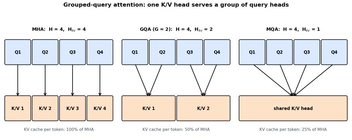
Three panels each showing four query head boxes above their key/value heads: MHA has four separate KV heads, GQA with group size two has two KV heads each fed by two query heads, and MQA has one KV head shared by all four query heads

Figure 1: The only structural change is how many distinct K/V heads exist; query heads are never merged, so each still has its own projection and its own attention pattern over the shared keys.

Mathematical Formulation:
$H_{kv} = H / G$
$g(i) = \lfloor i / G \rfloor$
$M_{tok} = 2 L H_{kv} d_h b$
$W_K^{(g)} = \frac{1}{G} \sum_{i \in \mathcal{G}_g} W_K^{(i)}$

Where:

$H$ is the number of query heads, $G$ the group size, and $H_{kv}$ the resulting number of key/value heads; $G = 1$ recovers MHA and $G = H$ recovers MQA.
$i \in \{0,\ldots,H-1\}$ indexes query heads and $g(i)$ is the KV head that head $i$ reads, so heads are assigned to groups by contiguous blocks.
$M_{tok}$ is the KV cache bytes per token, with $L$ layers, head dimension $d_h$ , bytes per element $b$ , and the factor 2 covering K and V; total cache is $M_{tok}$ times batch times sequence length.
$\mathcal{G}_g$ is the set of query-head indices in group $g$ , and the last line is the mean-pooling initialization used when converting an MHA checkpoint; the same averaging is applied to $W_V$ .

The payoff is easiest to see with a concrete configuration. A Llama-3-70B-shaped model has $L = 80$ , $H = 64$ , and $d_h = 128$ ; in FP16 that is 2.5 MiB per token of KV cache under MHA, 320 KiB under GQA with 8 KV heads, and 40 KiB under MQA. At a 32K context and batch size 1 those become 85.9 GB, 10.7 GB, and 1.34 GB. On a single H100 with 3.35 TB/s of HBM bandwidth, reading a 10.7 GB cache once costs roughly 3.2 ms per decoded token against roughly 26 ms for the 85.9 GB version; tensor parallelism divides both numbers, but the ratio is fixed by $H_{kv}$ and does not improve with more hardware. That freed memory is also what lets a server hold many more concurrent sequences, which is usually a larger throughput win than the per-token latency itself.

Log-scale bar chart of FP16 KV cache size at 32K context for a 70B-shaped model: MHA with 64 KV heads needs 85.9 GB, GQA with 8 KV heads needs 10.7 GB, and MQA with 1 KV head needs 1.34 GB, with a dashed line marking 80 GB of H100 HBM

Figure 2: FP16 KV cache for one 32K-token sequence on an 80-layer, 64-head, 128-dim model. Under MHA the cache alone would consume an entire 80 GB H100 before any weights are loaded.

Property	MHA	GQA (8 KV heads)	MQA
KV heads	64 (one per query head)	8 (group size 8)	1 (shared by all)
Cache per token (FP16)	2.5 MiB	320 KiB	40 KiB
Decode speed	Slowest, bandwidth bound on the cache	Close to MQA at long context	Fastest
Quality	Reference	Within noise of MHA on most benchmarks	Measurable drop, notably on long-input summarization
Tensor parallelism	Shards cleanly	Shards cleanly when $H_{kv}$ equals the shard count	KV must be replicated on every shard
Training stability	Stable baseline	Stable; uptrainable from an MHA checkpoint	Reported instability at scale

August 15, 2026

DL0075 Attention Sink

What is an attention sink, and why do models attend to the first token so heavily?

Answer

An attention sink is a token that a head dumps its attention mass onto when it has nothing relevant to retrieve, and in decoder-only LLMs that token is almost always the first one in the sequence (often the BOS token). Measured on a trained model, a middle-layer head can place well over half of its probability on that single position even though its value vector carries almost no task-relevant content. The cause is structural rather than semantic: softmax normalizes every attention row to sum to exactly 1, so a head has no way to say “attend to nothing” and must put the leftover mass somewhere. Causal masking makes the first token the only key visible from every query position, and it is the one token whose representation is not yet mixed with context, so training converges on it as the default no-op target. The model then reinforces the arrangement by growing massive activations and unusually large key norms at that position, which is why the sink shows up as an outlier in both attention maps and activation histograms.

(1) Softmax Has No No-Op: the row constraint $\sum_j \alpha_{ij} = 1$ means an idle head still emits a full distribution, so the mass must land on some low-cost token.
(2) Why The First Token Wins: under causal masking it is the only key every query can see, and it precedes all content, so it is both universally available and information-free, the ideal dumping ground.
(3) The Sink Is Load-Bearing: it is not decorative; drop the first token from a sliding-window KV cache and perplexity jumps by one to two orders of magnitude, because every head loses its default target and redistributes mass onto real tokens.
(4) Fingerprints Beyond Attention: the same position carries hidden-state outliers that widen activation ranges, which is a known headache for per-tensor quantization; vision transformers show the analogous effect by repurposing background patches as sinks.

Log-scale bar chart of attention mass by key position for one head at query position 512: token 0 receives 0.42, tokens 1 to 3 receive 0.06, 0.03 and 0.02, three middle bins receive 0.07, 0.06 and 0.09, and the most recent 64 positions receive 0.25

Figure 1: Illustrative single head at query position 512: the first token absorbs 0.42 of the mass, the most recent 64 positions share 0.25, and the roughly 444 middle positions split only 0.22, about $5\times 10^{-4}$ each.

The cleanest way to read the sink is as a learned bias term smuggled into the softmax. Because the denominator sums over all visible keys, the only way for a head to shrink the weight it gives to real tokens is to inflate the score of some other key; the first token, whose value vector contributes near-zero to the output, is that escape valve. This also explains the standard fixes. Giving the softmax an explicit extra term in the denominator (the off-by-one softmax, or a learned per-head sink logit as used in some recent open-weight models such as OpenAI’s gpt-oss) lets attention rows sum to less than 1, so no real token needs to be sacrificed. Prepending dedicated register tokens achieves the same thing with ordinary softmax by supplying a scratch position, which is what cleaned up the noisy attention maps in vision transformers. Both changes must be present during pretraining: retrofitting them onto a model that already routes mass through token 0 changes the normalization the weights were trained under.

Mathematical Formulation:
$s_{ij} = \frac{q_i^{\top} k_j}{\sqrt{d_k}}$
$\alpha_{ij} = \frac{\exp(s_{ij})}{\sum_{m=1}^{i} \exp(s_{im})}$
$\sum_{j=1}^{i} \alpha_{ij} = 1$
$\tilde{\alpha}_{ij} = \frac{\exp(s_{ij})}{\exp(b_h) + \sum_{m=1}^{i} \exp(s_{im})}$

Where:

$s_{ij}$ is the scaled dot-product score between query $q_i$ and key $k_j$ , with head dimension $d_k$ .
$\alpha_{ij}$ is the attention weight; $i$ indexes query positions and $j, m$ index key positions, restricted to $m \leq i$ by causal masking, which is why $j = 1$ is the only key shared by every query.
The third line is the normalization constraint that creates the sink: no configuration of scores lets a head emit less than one unit of total mass.
$b_h$ is a learned per-head sink logit added to the denominator, so $\sum_j \tilde{\alpha}_{ij}$ can fall below 1; the off-by-one softmax is the special case $b_h = 0$ , since $\exp(0) = 1$ .

Log-scale perplexity versus tokens streamed for three attention policies: dense attention rises past the 4096-token pretraining length, sliding-window attention jumps from about 10 to nearly 400 once the first token is evicted at 1024 tokens, and a window that retains 4 sink tokens stays flat near 10.5

Figure 2: Illustrative streaming behavior: a plain sliding window collapses the moment the first token leaves the KV cache, while retaining a handful of sink tokens alongside the window keeps perplexity flat far beyond the pretraining length.

Approach	What It Changes	Training Cost	When to Reach for It
Dense Attention	Nothing; the sink stays at token 0 and is never evicted	None	Short contexts where the full KV cache fits
Keep First k Tokens (StreamingLLM)	Cache policy only: pin the first 4 tokens plus a sliding window	None, works on an already-trained model	Streaming or long-running serving with a fixed cache budget
Register or Sink Tokens	Prepends learnable scratch tokens that heads can dump onto	Pretraining or substantial fine-tuning	New models, and ViTs whose attention maps must stay interpretable
Learned Sink Logit / Softmax Off-by-One	Extra denominator term so a row can sum to less than 1	Must be present from pretraining	New architectures, especially where activation outliers hurt quantization

August 14, 2026

DL0074 GRU vs LSTM

How does a GRU differ from an LSTM, and when would you prefer one over the other?

Answer

Both are gated recurrent cells that replace the vanilla RNN’s repeated multiplication by an additive state update, which is what keeps gradients alive across long sequences. The LSTM carries two state tensors (the cell state $c_t$ and the hidden state $h_t$ ) and three gates: forget, input, and output. The GRU is a leaner reparameterization that keeps one state: it merges forget and input into a single update gate $z_t$ whose two branches are tied as $z_t$ and $1 - z_t$ , deletes the output gate so the full state is exposed to the next layer, and adds a reset gate $r_t$ that suppresses the previous state inside the candidate. The practical consequence is three weight blocks instead of four, so roughly 25% fewer recurrent parameters and matmuls per step, plus one less tensor to carry and initialize. Accuracy is usually close (Chung et al. 2014; Greff et al. 2017), so the choice is driven by data size, latency, and whether the task needs the LSTM’s unbounded memory.

(1) Gate Inventory: LSTM has forget, input, and output gates; the GRU has update and reset only, because tying the write and erase decisions into $z_t$ and $1 - z_t$ removes one gate and dropping the output gate removes another.
(2) One State vs Two: the LSTM’s protected cell state $c_t$ is never squashed on the recurrent path and is only revealed through the output gate, while the GRU’s single $h_t$ is both the memory and the emitted representation.
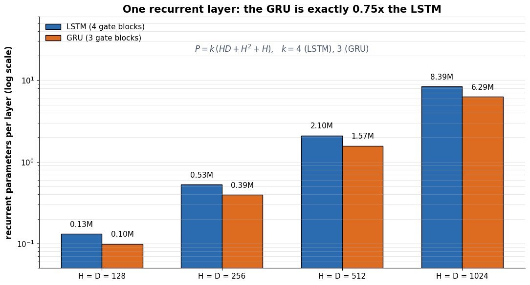
(3) Parameter and Compute Ratio: with input width $D$ and hidden width $H$ , the GRU costs exactly $3/4$ of the LSTM’s recurrent parameters and per-step FLOPs, which matters most when the recurrent stack dominates the model.
(4) Expressivity Gap: at finite precision, the LSTM’s additive, unsquashed cell state can implement a genuine counter, whereas the GRU’s convex-combination update keeps the state inside $[-1,1]$ and can only approximate counting (Weiss et al. 2018).
(5) How to Choose: prefer the GRU for small or medium datasets, short-to-medium sequences, and tight latency or memory budgets; prefer the LSTM for long sequences, large corpora, and tasks that need precise long-horizon bookkeeping such as language modeling.

Two side-by-side cell diagrams: the LSTM panel shows a cell-state track with multiply and add operators fed by forget and input gates plus an output gate producing h_t; the GRU panel shows a single hidden-state track with an update gate feeding both branches and a reset gate feeding the candidate

Figure 1: The LSTM keeps a separate cell-state track written by forget and input gates and read out through an output gate; the GRU folds everything onto one hidden-state track, where the update gate supplies both mixing weights and the reset gate only conditions the candidate.

Mathematical Formulation:
$c_t = f_t \odot c_{t-1} + i_t \odot \tilde{c}_t$
$h_t = o_t \odot \tanh(c_t)$
$\tilde{h}_t = \tanh(W_h x_t + r_t \odot U_h h_{t-1} + b_h)$
$h_t = (1 - z_t) \odot \tilde{h}_t + z_t \odot h_{t-1}$
$P_{\mathrm{LSTM}} = 4(HD + H^2 + H)$
$P_{\mathrm{GRU}} = 3(HD + H^2 + H)$

Where:

$h_t$ is the hidden state emitted at step $t$ and $c_t$ the LSTM’s internal cell state; both start from zero at $t = 0$ .
$x_t$ is the input at step $t$ , with $D$ its width and $H$ the hidden width.
$f_t, i_t, o_t$ are the LSTM forget, input, and output gates and $\tilde{c}_t$ its candidate, each of the form $\sigma(Wx_t + Uh_{t-1} + b)$ (with $\tanh$ for the candidate).
$z_t$ and $r_t$ are the GRU update and reset gates, both sigmoid, and $\tilde{h}_t$ is its candidate state.
$\odot$ is the elementwise product, $\sigma$ the logistic sigmoid mapping to $(0,1)$ , and $W, U, b$ the input, recurrent, and bias parameters of one gate block.
$P$ counts recurrent-cell parameters only, so the ratio $P_{\mathrm{GRU}}/P_{\mathrm{LSTM}} = 3/4$ holds for any $D$ and $H$ .

Grouped bar chart on a log scale of recurrent parameter counts for hidden widths 128, 256, 512 and 1024 with input width equal to hidden width: LSTM bars are 0.13M, 0.53M, 2.10M and 8.39M while GRU bars are 0.10M, 0.39M, 1.57M and 6.29M

Figure 2: Recurrent parameters per layer with $D = H$ : three gate blocks instead of four give the GRU exactly 0.75x the LSTM count at every width, so at $H = 512$ one layer holds 1.57M against 2.10M.

Property	GRU	LSTM
Gates	2: update, reset	3: forget, input, output
State carried	Hidden state only	Hidden state plus cell state
Weight blocks	3	4
Params at D = H = 512	1.57M	2.10M
Memory exposure	Whole state is exposed downstream	Output gate filters what leaves the cell
Unbounded counting	No: state stays bounded by the convex update	Yes: additive, unsquashed cell state
Where it tends to win	Small data, short sequences, tight latency	Long sequences, large corpora, language modeling

August 14, 2026

DL0073 EfficientNet Compound Scaling
How does EfficientNet scale networks, and what is compound scaling?
Answer
EfficientNet starts from a small baseline, EfficientNet-B0, produced by a multi-objective architecture search that rewards accuracy and FLOPs together, and then grows that fixed topology into the family B1 through B7 by scaling three dimensions simultaneously: depth (number of layers), width (number of channels), and input resolution. The empirical observation behind the method is that scaling any single dimension saturates: beyond a point, extra layers, extra channels, or extra pixels buy almost no accuracy while still costing compute. Compound scaling ties the three together through one user-chosen coefficient $\phi$ and three fixed exponents $\alpha, \beta, \gamma$ obtained by a small grid search on B0, subject to $\alpha \cdot \beta^{2} \cdot \gamma^{2} \approx 2$ so that each unit of $\phi$ roughly doubles the FLOPs budget. With $\alpha = 1.2$ , $\beta = 1.1$ , $\gamma = 1.15$ , the family climbs from 77.1% ImageNet top-1 at 0.39B FLOPs (B0) to 84.3% at 37B FLOPs (B7), matching the best accuracy of its era with about 8.4x fewer parameters than GPipe.
(1) The Baseline Is a Prerequisite: compound scaling only multiplies an existing topology, so a weak baseline yields a weak family; B0 is itself a search result built from MBConv blocks with squeeze-and-excitation, and the same scaling rule applied to MobileNet or ResNet gives smaller gains.
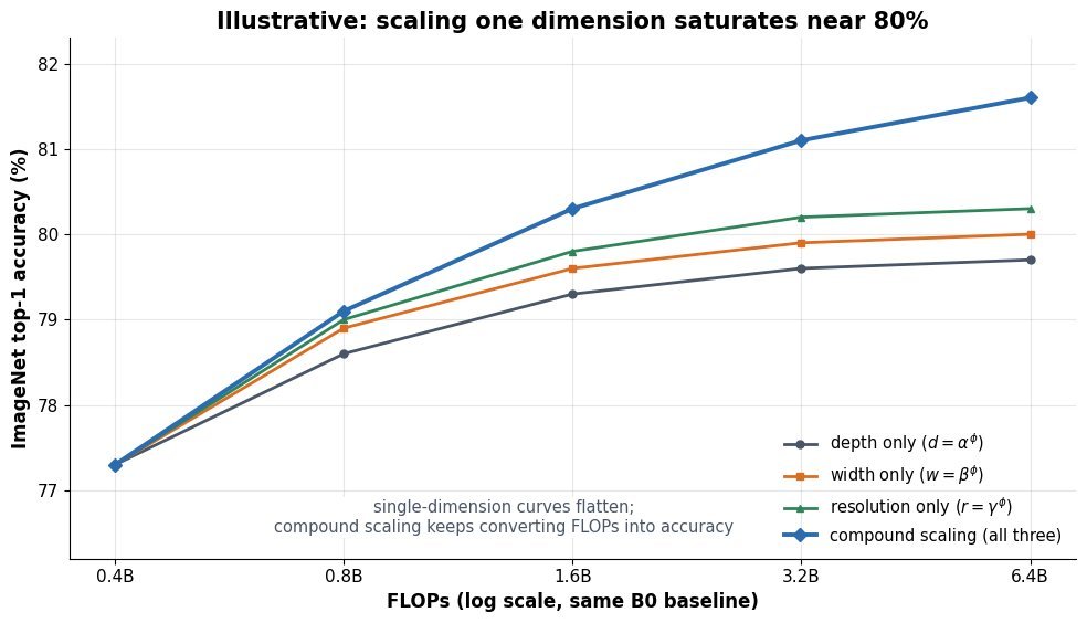
(2) Single-Dimension Scaling Saturates: very deep networks hit optimization and degradation limits, very wide shallow networks capture fine-grained patterns but few high-level ones, and resolution alone raises cost quadratically for shrinking returns.
(3) The Balance Rule: a larger input needs more layers to grow the receptive field and more channels to encode the finer patterns those extra pixels expose, which is why the three factors should move in a fixed ratio rather than one at a time.
(4) Two-Step Search: fix $\phi = 1$ and grid-search $\alpha, \beta, \gamma$ once on the cheap baseline, then freeze them and sweep $\phi$ to get B1 through B7, which avoids re-searching the architecture at every model size.

Figure 1: Illustrative accuracy-versus-compute curves from the same B0 baseline: depth-only, width-only, and resolution-only scaling flatten near 80% top-1, while compound scaling keeps converting FLOPs into accuracy.
The constraint has a direct cost interpretation. A standard convolution’s FLOPs scale linearly with the number of layers and quadratically with both channel count and spatial size, so total compute grows like $d \cdot w^{2} \cdot r^{2}$ . Forcing $\alpha \cdot \beta^{2} \cdot \gamma^{2} \approx 2$ therefore makes $\phi$ a clean compute dial: each additional unit costs about 2x the FLOPs, and the exponents decide how that doubled budget is split across the three dimensions. The exponents are searched once, on a model cheap enough that a small grid over $\alpha, \beta, \gamma$ is affordable.
Mathematical Formulation:
$d = \alpha^{\phi}$
$w = \beta^{\phi}$
$r = \gamma^{\phi}$
$\alpha \cdot \beta^{2} \cdot \gamma^{2} \approx 2$
$\mathrm{FLOPs}(\phi) \approx 2^{\phi} \cdot \mathrm{FLOPs}(0)$
Where:
$d$ , $w$ , and $r$ are the multipliers applied to the baseline’s layer count per stage, channel count per layer, and input side length.
$\phi$ is the user-chosen compound coefficient that sets the resource budget; $\phi = 0$ recovers the baseline B0.
$\alpha, \beta, \gamma$ are constants from a small grid search on B0 with $\alpha \geq 1$ , $\beta \geq 1$ , $\gamma \geq 1$ ; the published values are $1.2$ , $1.1$ , and $1.15$ .
Convolution cost scales as $d \cdot w^{2} \cdot r^{2}$ , so the product constraint is what turns $\phi$ into an approximate doubling of FLOPs per unit.

Figure 2: The same topology at two budgets: a bigger input square (resolution), taller blocks (width), and more blocks (depth) all grow together instead of one dimension racing ahead.
Model Depth Width Resolution FLOPs ImageNet Top-1
B0 1.0x 1.0x 224 0.39B 77.1%
B3 1.4x 1.2x 300 1.8B 81.6%
B5 2.2x 1.6x 456 9.9B 83.6%
B7 3.1x 2.0x 600 37B 84.3%
Two caveats matter in practice. The released coefficients are rounded rather than exact powers of a single $\phi$ , so treat the formula as the design principle and the published table as the shipped configuration. More importantly, the objective is FLOPs, not latency or memory: depthwise separable convolutions have low arithmetic intensity and underuse GPU and TPU matrix units, and activation memory grows with $r^{2}$ , so the largest variants train slowly and can exhaust device memory. EfficientNetV2 addressed exactly this by replacing early MBConv stages with Fused-MBConv, capping the maximum image size, and adding training-aware search plus progressive resizing.
Login to view more content
August 14, 2026

Model	Depth	Width	Resolution	FLOPs	ImageNet Top-1
B0	1.0x	1.0x	224	0.39B	77.1%
B3	1.4x	1.2x	300	1.8B	81.6%
B5	2.2x	1.6x	456	9.9B	83.6%
B7	3.1x	2.0x	600	37B	84.3%

DL0072 Inception Module

What is the Inception module, and how does it use parallel convolutions of different sizes?

Answer

The Inception module is the building block of GoogLeNet: instead of committing a layer to one kernel size, it runs several convolutional branches in parallel over the same input (1×1, 3×3, 5×5, plus a 3×3 max-pool path) and concatenates their outputs along the channel axis. Every branch uses stride 1 with padding chosen so all branches emit the same spatial size, which is what makes the concatenation legal. The naive form is prohibitively expensive because the 5×5 branch convolves over the full input depth, so the practical module inserts 1×1 convolutions as channel bottlenecks before the 3×3 and 5×5 convolutions and after the pooling path. The next layer therefore sees features at several receptive-field sizes at once, and the learned weights decide how much of each scale to use rather than the architect fixing one kernel per layer.

(1) Parallel Multi-Scale Branches: the 1×1, 3×3, 5×5, and pooling paths all read the identical input tensor, so one module covers several receptive fields; a face at 20 px and one at 60 px are both matched inside the same layer.
(2) Channel-Wise Concatenation: branches keep $H$ and $W$ identical (stride 1, pad 1 for 3×3, pad 2 for 5×5), and outputs are stacked on the channel dimension, so module output depth is the sum of branch depths, not their average.
(3) 1×1 Bottlenecks: convolution cost is linear in $C_{in} C_{out} k^2$ , so projecting 192 channels down to 16 before the 5×5 conv cuts that branch roughly 10x with a small accuracy cost.
(4) Dense Ops, Sparse Intent: the design approximates a sparse, locally-optimal connectivity structure using dense operations that BLAS and cuDNN execute efficiently, which is why GoogLeNet reached top ILSVRC-2014 accuracy at about 5M parameters, roughly 12x fewer than AlexNet.

Two side-by-side block diagrams of an Inception module: on the left the naive version sends the 28x28x192 input straight into 1x1, 3x3, 5x5 convolutions and a 3x3 max pool before filter concatenation; on the right the dimension-reduced version inserts 1x1 convolutions with 96 and 16 channels before the 3x3 and 5x5 convolutions and a 32-channel 1x1 projection after the pool

Figure 1: Naive versus dimension-reduced Inception module. The 1×1 convolutions shrink channel depth before the expensive kernels and project the pooled path, so concatenation does not grow depth without bound.

The pooling branch is the reason the naive module is unstable when stacked: max pooling preserves its input depth, so every module would add at least the full input depth back into the concatenated output and channel count would grow monotonically with depth. The 1×1 projection after the pool fixes this, and the same trick applied before the 3×3 and 5×5 convolutions is where nearly all the savings come from. Take the classic Inception (3a) block with a $28 \times 28 \times 192$ input and a 5×5 branch producing 32 maps.

Mathematical Formulation:
$y = \mathrm{concat}(y_1, y_3, y_5, y_p)$
$C = H_o W_o C_{out} k^2 C_{in}$
$C_{naive} = 28^2 \cdot 32 \cdot 5^2 \cdot 192 \approx 120 \times 10^6$
$C_{reduce} = 28^2 \cdot 16 \cdot 1^2 \cdot 192 \approx 2.4 \times 10^6$
$C_{conv} = 28^2 \cdot 32 \cdot 5^2 \cdot 16 \approx 10.0 \times 10^6$

Where:

$y_1, y_3, y_5, y_p$ are the outputs of the 1×1, 3×3, 5×5, and pooling branches, and $\mathrm{concat}$ stacks them on the channel axis, which requires all four to share the same $H_o \times W_o$ .
$C$ counts multiply-adds for one convolution, with $H_o W_o$ the output spatial size, $C_{in}$ and $C_{out}$ the input and output channels, and $k$ the kernel width.
$C_{naive}$ is the 5×5 branch applied to all 192 input channels; $C_{reduce}$ is the 1×1 projection to 16 channels and $C_{conv}$ the 5×5 conv on those 16, summing to about $12.4 \times 10^6$ , roughly a tenth of the naive branch.

Grouped bar chart of multiply-adds in millions per Inception 3a branch, naive versus dimension-reduced: 1x1 branch 9.6 and 9.6, 3x3 branch 173.4 and 101.2, 5x5 branch 120.4 and 12.4, pool branch 0 and 4.8, module total 303.5 and 128.0

Figure 2: Multiply-adds per branch for Inception (3a) on a $28 \times 28 \times 192$ input. The bottlenecks cut the 5×5 branch from about 120M to 12M and the module total from about 304M to 128M, while also shrinking output depth from 416 to 256 channels.

Branch	1×1 Reduction	Main Operation	Output Channels	Multiply-Adds
Point-wise	none needed	1×1 conv, 64 filters	64	9.6M
Medium scale	192 to 96	3×3 conv, 128 filters, pad 1	128	101.2M
Large scale	192 to 16	5×5 conv, 32 filters, pad 2	32	12.4M
Pooling	192 to 32, after the pool	3×3 max pool, stride 1, pad 1	32	4.8M
Concatenated	–	channel-axis concat, 28×28 preserved	256	128M

August 14, 2026

DL0071 VGG vs GoogLeNet vs ResNet

Compare VGG, GoogLeNet/Inception, and ResNet: what key problem did each architecture address?

Answer

The three architectures answer three different questions that the ImageNet era asked in sequence. VGG (2014) asked whether depth alone helps and showed that stacking small 3×3 convolutions to 16 or 19 weight layers beats wide shallow filters, but it paid for that with 138M parameters and 15.3 GFLOPs, roughly 90% of the parameters sitting in three fully connected layers. GoogLeNet/Inception (2014) asked how to get depth and multi-scale receptive fields cheaply: parallel 1×1, 3×3, 5×5, and pooling branches inside one Inception module, with 1×1 bottleneck convolutions cutting channel depth before the expensive kernels, plus global average pooling replacing the fully connected head, giving better accuracy than VGG with about 6.8M parameters and 1.5 GFLOPs. ResNet (2015) asked why depth stopped paying off past roughly 20 to 30 layers and identified the degradation problem: a 56-layer plain net reaches higher training error than a 20-layer one, so this is an optimization failure, not overfitting. Its fix, the identity shortcut $y = \mathcal{F}(x) + x$ , makes each block learn a residual and gives gradients a direct path, which made 152-layer and even 1000-layer networks trainable.

(1) VGG, Depth Through Uniformity: three stacked 3×3 layers match the 7×7 receptive field with fewer parameters and two extra nonlinearities, proving that a simple repeated motif scales; the cost is a parameter-heavy fully connected head and no answer to what happens beyond ~19 layers.
(2) Inception, Depth Under a Compute Budget: the module runs several kernel sizes in parallel so the network does not have to choose one scale per layer, and 1×1 reduce → 5×5 conv keeps the cost of the wide branches roughly an order of magnitude lower than the naive version.
(3) ResNet, Depth Without Degradation: residual blocks reframe the layer’s job as learning a correction to identity, so adding layers can never be worse than copying the input; combined with batch normalization and bottleneck blocks (1×1, 3×3, 1×1), it made very deep training routine.

Parameter Arithmetic:
$3 \times 3^2 C^2 = 27 C^2$
$1 \times 7^2 C^2 = 49 C^2$
$5^2 \cdot 192 \cdot 32 = 153{,}600$
$192 \cdot 16 + 5^2 \cdot 16 \cdot 32 = 15{,}872$

Where:

$C$ is the channel count held constant across the stack, so the first two lines compare three 3×3 layers against one 7×7 layer of identical receptive field: about 45% fewer weights and two extra ReLUs.
The third line is the naive Inception 5×5 branch: 192 input channels, 32 output channels, $5^2$ spatial taps.
The fourth line inserts a 1×1 reduce to 16 channels first, so the same branch costs 15,872 weights, roughly $10\times$ cheaper; this bottleneck is what let GoogLeNet run 22 layers at 1.5 GFLOPs.

Scatter plot of ImageNet top-5 error against parameter count on a log scale for VGG-16 at 138M parameters and 7.3 percent, GoogLeNet at 6.8M and 6.7 percent, ResNet-50 at 25.6M and 5.25 percent, and ResNet-152 at 60.2M and 4.49 percent

Figure 1: Accuracy did not come from parameter count: GoogLeNet beats VGG-16 with about $20\times$ fewer parameters, and ResNet improves again at moderate size. Evaluation protocols differ slightly across the original papers, so read the trend rather than the decimals.

The residual idea is the one that generalized furthest. Writing a block as $y = \mathcal{F}(x, \{W_i\}) + x$ means the optimizer only has to push $\mathcal{F}$ toward zero to recover the identity mapping, which is exactly the solution the deeper plain net failed to find. The gradient view is just as important: the identity term contributes an ungated path so the signal reaching early layers cannot vanish through repeated multiplication by small Jacobians. In practice the projection shortcut ( $1\times1$ convolution with stride 2) handles the stage boundaries where spatial size and channel count change.

Residual Formulation:
$y = \mathcal{F}(x, \{W_i\}) + x$
$\frac{\partial L}{\partial x} = \frac{\partial L}{\partial y}\left(I + \frac{\partial \mathcal{F}}{\partial x}\right)$

Where:

$x$ is the block input, $y$ its output, and $\mathcal{F}$ the two or three stacked convolutions with weights $\{W_i\}$ .
$I$ is the identity Jacobian of the shortcut; it keeps the gradient norm from collapsing even when $\partial \mathcal{F} / \partial x$ is tiny, which is why depth beyond 100 layers becomes trainable.
$L$ is the training loss; when shapes differ across a stage, $x$ is replaced by $W_s x$ with a projection shortcut.

Schematic training error curves over 160 epochs: a 56-layer plain network plateaus at a higher training error than a 20-layer plain network, while a 56-layer ResNet reaches the lowest training error

Figure 2: Schematic of the degradation problem: the deeper plain network settles at higher training error than the shallower one, ruling out overfitting; the residual version of the same depth trains to the lowest error.

Aspect	VGG (2014)	GoogLeNet / Inception (2014)	ResNet (2015)
Key problem addressed	Does depth with small kernels beat shallow wide kernels?	How to buy depth and multiple scales on a fixed compute budget	Degradation: deeper plain nets train worse
Signature component	Uniform 3×3 conv stacks plus 2×2 max pool	Inception module with 1×1 bottlenecks, global average pooling	Identity shortcut, bottleneck block (1×1, 3×3, 1×1), batch norm
Depth	16 or 19 weight layers	22 layers	18 to 152, and 1000+ in experiments
Parameters / compute	138M, 15.3 GFLOPs	~6.8M, 1.5 GFLOPs	25.6M, 3.8 GFLOPs (ResNet-50)
Main drawback	Huge FC head, memory hungry, stalls past ~19 layers	Hand-tuned, irregular module; harder to modify or scale	Still heavy for edge devices; deep variants give diminishing returns
Lasting legacy	3×3 as the default kernel; perceptual loss backbone	1×1 channel bottlenecks; no-FC classification heads	Residual connections in nearly every modern net, including Transformers

August 14, 2026