Author: admin

ML0093 DBSCAN Clustering

How does DBSCAN work, and what advantages does it have over k-means for clustering tasks like geospatial stop detection?

Answer

DBSCAN is a density-based clustering algorithm: it groups points that are packed closely together and labels isolated points as noise, all without being told how many clusters to find. For each point it counts how many points fall within a radius eps; any point whose eps-neighborhood holds at least min_samples points (counting itself) is a core point, and clusters grow by linking core points whose neighborhoods overlap, then attaching their non-core neighbors. K-means, by contrast, requires you to specify K upfront and partitions data into Voronoi cells around centroids, which forces spherical clusters and assigns every point somewhere even if it is an outlier. In geospatial applications, DBSCAN is used to cluster raw GPS pings into “stops” because the density-based approach naturally absorbs GPS jitter and ignores transient traffic halts without needing a predefined polygon count.

(1) Density-Connected Expansion: a cluster is the maximal set of density-reachable points from a core point; points with fewer than min_samples neighbors but inside a core’s eps-radius become border points, and points reachable from no core become noise.
(2) No K and Arbitrary Shapes: DBSCAN discovers the cluster count from the data and follows winding, non-convex boundaries, which k-means cannot do because its Voronoi partition assumes spherical, similarly sized groups.
(3) Production Pattern: geospatial pipelines chain DBSCAN then SVM on GPS streams for foot-traffic analysis, and embedding-based clustering pairs UMAP with HDBSCAN (hierarchical DBSCAN) for recursive clustering because it handles varying densities and auto-selects stable clusters without an eps parameter.

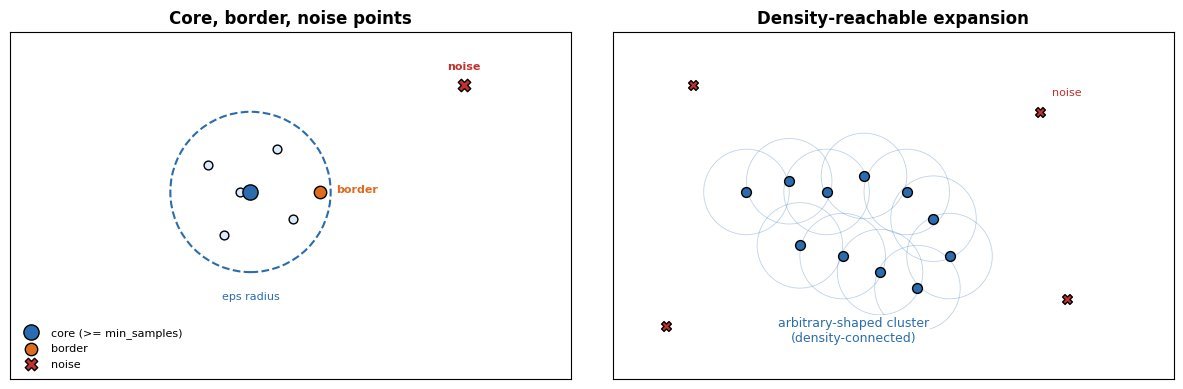
Left panel: DBSCAN core point with eps-radius circle and min_samples neighbors, a border point on the circle edge, and a noise point outside; right panel: density-reachable expansion linking core points into an arbitrary-shaped cluster

Figure 1: DBSCAN mechanics: a core point has at least min_samples neighbors inside the eps-radius circle; clusters expand by chaining overlapping core neighborhoods, border points attach to one cluster, and isolated points become noise.

The practical trade-off is parameter sensitivity and density variation. DBSCAN’s eps must be tuned to the data’s scale, and a single global eps struggles when clusters have different densities, which is why HDBSCAN extends DBSCAN into a hierarchy and extracts stable clusters at varying density levels. K-means is cheaper at scale (each iteration is O(nKd) and embarrassingly parallel) and wins when clusters are genuinely spherical and K is known, as in vector quantization for image compression. DBSCAN’s neighborhood queries cost O(n log n) with a spatial index but degrade to O(n^2) in high dimensions where indexing breaks down, so production pipelines reduce dimensionality with UMAP first.

Two side-by-side panels on the same two-moon dataset: the left panel shows k-means cutting both moons with a straight dashed Voronoi boundary, the right panel shows DBSCAN recovering the two curved moons and marking sparse points as noise with gray crosses

Figure 2: On a non-convex two-moon dataset, k-means imposes a linear Voronoi cut that slices through both moons, while DBSCAN follows the curved density ridges and marks sparse-gap points as noise.

Mathematical Formulation:
$N_{\mathrm{eps}}(p) = \{q \in D \mid \mathrm{dist}(p, q) \leq \mathrm{eps}\}$
$\text{core}(p) \iff |N_{\mathrm{eps}}(p)| \geq \mathrm{min\_samples}$
$q \in C \iff \exists\, p_1, \ldots, p_t \in D:\ p_i \text{ core},\ p_{i+1} \in N_{\mathrm{eps}}(p_i),\ q \in N_{\mathrm{eps}}(p_t)$

Where:

$N_{\mathrm{eps}}(p)$ is the eps-neighborhood of point $p$ in dataset $D$ , and $\mathrm{dist}$ is typically Euclidean distance.
A point is core when its neighborhood contains at least min_samples points; border points are in a core’s neighborhood but are not core themselves; noise points are in no core’s neighborhood.
A cluster $C$ is the maximal set of points density-reachable from a core point via a chain of overlapping core neighborhoods; this transitive closure is what lets DBSCAN trace arbitrary shapes.

Property	DBSCAN	k-means
Cluster Count	Discovered from density; no K needed	Must specify K upfront
Cluster Shape	Arbitrary, density-connected	Spherical Voronoi cells
Outliers	Labeled as noise explicitly	Force-assigned to nearest centroid
Parameters	eps, min_samples	K, initialization
Scalability	O(n log n) with spatial index; O(n^2) worst case	O(nK) per iteration, parallelizable
Weakness	Single eps fails on varying densities (HDBSCAN fixes this)	Breaks on non-spherical or unequal-size clusters

August 12, 2026

ML0092 Naive Bayes for Continuous Features

How does Naive Bayes handle continuous numeric features, and what goes wrong when the Gaussian assumption is violated?

Answer

The default approach is Gaussian Naive Bayes: for each continuous feature, the model estimates a per-class mean and variance from the training data and plugs the feature value into the Gaussian PDF to get the likelihood. This is fast (one pass to compute mean and variance, O(nd)) and works well when features are approximately normal within each class, as in the Iris dataset or standardized medical lab values. The problem is that the Gaussian assumption is often violated: income is right-skewed, reaction times are log-normal, and sensor readings can be multi-modal. When the true distribution is skewed or has heavy tails, the Gaussian likelihood misestimates the probability mass, pushing the posterior toward 0 or 1 incorrectly. The fixes are discretization (bin the feature and use Categorical or Multinomial NB), kernel density estimation (replace the parametric Gaussian with a non-parametric KDE), or transformation (log or Box-Cox transform to normalize the feature before applying Gaussian NB).

(1) Gaussian NB (Default): estimates $\mu_{yj}$ and $\sigma_{yj}^2$ per class per feature, then uses the Gaussian PDF in the likelihood product; O(nd) training, O(d) prediction, but assumes normality.
(2) Discretization: bin the continuous feature into k bins (equal-width or quantile), then treat it as categorical with k values; the 2024 Max-Relevance-Min-Divergence (MRmD) method beats prior discretization schemes on most of 45 benchmark datasets by maximizing discriminant information and generalization simultaneously.
(3) Kernel Density Estimation: replace the Gaussian with a non-parametric KDE $\hat{f}(x \mid y) = \frac{1}{n_y h}\sum K(\frac{x - x_i}{h})$ ; the R naivebayes package and MATLAB’s ClassificationNaiveBayes both support it, and a 2025 paper used optimized robust KDE with Welsch M-estimation to handle outliers in Bayesian classification.

Three panels: left shows a skewed income distribution with a Gaussian fit that misses the long tail; middle shows discretization into bins with per-class bin probabilities; right shows a KDE curve that follows the true skewed shape closely

Figure 1: Three approaches to continuous features in Naive Bayes: Gaussian NB fits a normal curve that misses skewness, discretization bins the feature into categorical probabilities, and kernel density estimation follows the true non-parametric shape.

The practical decision flow is: start with Gaussian NB and check the per-class histograms. If the feature is approximately normal within each class, Gaussian is fine and is the cheapest option. If the feature is skewed but unimodal, apply a log or Box-Cox transform and re-check normality. If the feature is multi-modal or has heavy tails that resist transformation, use discretization (simpler, faster, but loses information) or KDE (more accurate, but slower at prediction because it evaluates the kernel against all training points in that class). Scikit-learn’s GaussianNB also tends to produce overconfident probabilities because the independence assumption compounds with the Gaussian misfit, so CalibratedClassifierCV with isotonic regression is recommended when the predicted probabilities need to be reliable, as in a medical risk score where the probability itself (not just the classification) drives the decision.

Mathematical Formulation:
$P(x_j \mid y) = \frac{1}{\sqrt{2\pi\sigma_{yj}^2}} \exp\!\left(-\frac{(x_j - \mu_{yj})^2}{2\sigma_{yj}^2}\right)$
$\hat{f}_h(x \mid y) = \frac{1}{n_y h} \sum_{i=1}^{n_y} K\!\left(\frac{x - x_i^{(y)}}{h}\right)$

Where:

The first equation is Gaussian NB: $\mu_{yj}$ and $\sigma_{yj}^2$ are the class-conditional mean and variance of feature $j$ , estimated as the sample mean and variance of all training values of feature $j$ in class $y$ .
The second equation is kernel density estimation: $n_y$ is the number of training points in class $y$ , $h$ is the bandwidth, $K$ is the kernel function (typically Gaussian), and $x_i^{(y)}$ are the training values of the feature in class $y$ .
For discretization, the continuous range is split into $k$ bins, and $P(\text{bin}_b \mid y) = (N_{yb} + \alpha) / (N_y + \alpha k)$ with Laplace smoothing, reducing the continuous feature to a categorical one.

Method	Assumption	Training Cost	When to Use
Gaussian NB	Normal per class	O(nd) one pass	Approximately normal features (Iris, standardized labs)
Discretization	No distributional assumption	O(nd) binning + counting	Skewed, multi-modal, or heavy-tailed features
KDE	Non-parametric	O(nd) storage; O(n_y) per prediction	Arbitrary distributions where bandwidth can be tuned
Transform + Gaussian	Normal after transform	O(nd) transform + estimate	Log-normal, power-law features (income, reaction time)

August 12, 2026

ML0091 Naive Bayes Types

What are the different types of Naive Bayes classifiers (Gaussian, Multinomial, Bernoulli), and when is each appropriate for tasks like Microsoft’s spam filtering or medical diagnosis?

Answer

The three main variants of Naive Bayes differ in the distribution they assume for each feature given the class, and the choice is driven by the feature type. Gaussian Naive Bayes assumes each continuous feature follows a normal distribution per class, estimated by the class-conditional mean and variance; it suits real-valued features like medical lab values or sensor readings. Multinomial Naive Bayes models integer feature counts drawn from a multinomial distribution, and in practice TF-IDF weights are often substituted even though they are not counts; it is the standard for text classification, used in Microsoft’s spam filtering training module and production review-spam detection processing 85,000 reviews per day. Bernoulli Naive Bayes models binary presence/absence indicators with a Bernoulli distribution; it suits boolean features like “contains word X” or “has flag Y” and explicitly accounts for the absence of a feature, which Multinomial NB does not.

(1) Gaussian NB (Continuous): estimates $\mu_{yj}$ and $\sigma_{yj}^2$ per class per feature; best for real-valued features like blood pressure, age, or sensor readings; assumes normality, so skewed or multi-modal features need transformation or kernel density estimation.
(2) Multinomial NB (Count Data): estimates $P(w_j \mid y) = (N_{yj} + \alpha) / (N_y + \alpha d)$ ; the standard for text classification on word counts, and commonly run on TF-IDF weights as a practical approximation; Microsoft’s training module uses it for email spam filtering, and a production system classifies 85,000 reviews/day at AUC above 0.99.
(3) Bernoulli NB (Binary Presence): estimates $P(x_j = 1 \mid y)$ and explicitly models $P(x_j = 0 \mid y)$ ; best for short documents or boolean feature sets where absence is informative; scikit-learn ships it alongside categorical and complement variants, and the R naivebayes package adds a Poisson variant for count features.

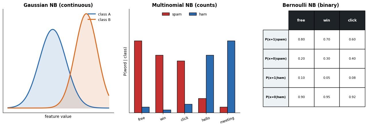
Three panels: Gaussian NB shows bell curves per class for a continuous feature; Multinomial NB shows a bar chart of word count probabilities per class; Bernoulli NB shows a binary presence/absence table with P(x=1|y) and P(x=0|y)

Figure 1: The three Naive Bayes variants: Gaussian models continuous features as per-class normal distributions, Multinomial models count data as a multinomial over a vocabulary, and Bernoulli models binary presence/absence with explicit absence probabilities.

The choice between Multinomial and Bernoulli for text depends on document length and whether absence carries information. Multinomial NB uses word frequencies, so a word appearing three times contributes three times the evidence; Bernoulli NB uses only presence, so “free” appearing once or ten times contributes the same amount, but the absence of “free” also contributes evidence. For long documents where frequency matters (emails, articles), Multinomial is standard. For short documents where presence is the signal (search queries, short reviews), Bernoulli can match or beat Multinomial. A common production pattern is TF-IDF weighting with Multinomial NB, as in the Banking77 support ticket router that classifies 13,000 banking queries into 77 intents in under 1 ms per ticket. For mixed feature types (continuous plus categorical plus binary), scikit-learn does not natively combine variants, so practitioners either discretize continuous features or use the R naivebayes package which supports mixed distributions including kernel density estimation.

Mathematical Formulation:
$P(x_j \mid y) = \frac{1}{\sqrt{2\pi\sigma_{yj}^2}} \exp\!\left(-\frac{(x_j - \mu_{yj})^2}{2\sigma_{yj}^2}\right)$
$P(x_j \mid y) = \frac{N_{yj} + \alpha}{N_y + \alpha\, d}$
$P(x_j \mid y) = \theta_{yj}^{x_j}(1 - \theta_{yj})^{1 - x_j}$

Where:

The first equation is Gaussian NB: $\mu_{yj}$ and $\sigma_{yj}^2$ are the mean and variance of feature $j$ in class $y$ , estimated from training data.
The second equation is Multinomial NB: $N_{yj}$ is the count of feature $j$ in class $y$ , $N_y$ is the total count, $\alpha$ is Laplace smoothing, and $d$ is the vocabulary size.
The third equation is Bernoulli NB: $\theta_{yj} = P(x_j = 1 \mid y)$ is the probability that feature $j$ is present in class $y$ ; the term $(1 - \theta_{yj})^{1 - x_j}$ explicitly models the absence of the feature.

Variant	Feature Type	Distribution	Best For
Gaussian NB	Continuous (real-valued)	Normal per class	Medical diagnosis, sensor data, Iris dataset
Multinomial NB	Counts or TF-IDF	Multinomial	Email spam, review classification, ticket routing
Bernoulli NB	Binary presence/absence	Bernoulli	Short text, boolean features, spam with word presence

August 12, 2026

ML0090 Naive Bayes Classifier

Explain the Naive Bayes classifier and the “naive” conditional independence assumption behind it, as used in production spam detection and support ticket routing.

Answer

Naive Bayes is a probabilistic classifier that applies Bayes’ theorem with a “naive” assumption: given the class label, all features are conditionally independent. This lets the classifier multiply per-feature likelihoods instead of estimating the full joint distribution, which would require exponential data. Despite the assumption being almost always violated in practice, Naive Bayes trains in O(nd) time, predicts in O(d) time, and performs surprisingly well on text classification, spam filtering, and support ticket routing. A production case study processes 85,000 product reviews per day with Multinomial Naive Bayes, achieving AUC above 0.99 for spam detection while retraining in under 5 minutes on a single-core VM, and a TF-IDF plus Multinomial NB pipeline routes banking support tickets in under 1 millisecond per ticket on the Banking77 dataset.

(1) Bayes’ Theorem Applied: the classifier computes the posterior $P(y \mid x)$ for each class and picks the argmax; the naive assumption factors the likelihood $P(x_1, \ldots, x_d \mid y)$ into a product of one-dimensional terms $\prod P(x_j \mid y)$ .
(2) Why the Assumption Works Anyway: even when the independence assumption is wrong, the argmax decision is often correct because correlated features push the posterior in the same direction; the calibration is off but the ranking is not, which is why scikit-learn recommends CalibratedClassifierCV with isotonic regression for reliable probabilities.
(3) Production Strengths: trains in milliseconds, predicts in microseconds, needs no GPU, produces interpretable per-feature contributions, and a 2024 Generalized Naive Bayes paper showed that relaxing the independence assumption via optimal structure learning improves accuracy while keeping the computational profile.

Two panels: left shows the full joint distribution P(x1,x2,x3|y) as a large table requiring exponential data; right shows the naive factorization as three small per-feature tables P(x1|y), P(x2|y), P(x3|y) multiplied together

Figure 1: The naive independence assumption factorizes the intractable joint likelihood P(x1, x2, x3 | y) into a product of one-dimensional per-feature likelihoods, replacing an exponential-size table with d small tables.

The independence assumption is the single most important thing to understand about Naive Bayes, because it is both its source of speed and its source of error. When two features are highly correlated (e.g., “free” and “gift” both appearing in spam), the classifier double-counts their evidence, pushing the posterior toward 0 or 1 more aggressively than the true joint distribution would. This is why GaussianNB in scikit-learn tends to produce overconfident probabilities and why calibration is recommended. The assumption also means Naive Bayes cannot capture feature interactions; a 2024 paper on Generalized Naive Bayes (GNB) addresses this by learning an optimal dependency structure among features while preserving the efficient factorization, proving the approximation is at least as good as classical Naive Bayes. For text specifically, the classic remedies are TF-IDF weighting, document-length normalization, and complement Naive Bayes, introduced by Rennie et al. to correct the multinomial model’s mismatch with real text. In practice, the speed-accuracy trade-off favors Naive Bayes for high-volume, low-latency text tasks where a transformer would be overkill.

Mathematical Formulation:
$\hat{y} = \arg\max_{y}\; P(y) \prod_{j=1}^{d} P(x_j \mid y)$
$P(x_j \mid y) = \frac{N_{yj} + \alpha}{N_y + \alpha\, d}$

Where:

$\hat{y}$ is the predicted class; $P(y)$ is the class prior, and the product of per-feature likelihoods replaces the intractable joint $P(x_1, \ldots, x_d \mid y)$ under the naive conditional independence assumption.
The second equation is the smoothed estimator for discrete (count) features: $N_{yj}$ is the count of feature $j$ in class $y$ , $N_y$ is the total count for class $y$ , $d$ is the vocabulary size, and $\alpha$ is the Laplace smoothing parameter (typically 1) that prevents zero probabilities for unseen feature-class combinations. Continuous features use a density instead, such as a per-class Gaussian.
The argmax is computed in log space to avoid underflow: $\log P(y) + \sum_j \log P(x_j \mid y)$ , which is a sum of precomputed log-likelihoods and runs in O(d) per prediction.

Property	Naive Bayes	Logistic Regression
Training Cost	O(nd) single pass	O(nd) per iteration, multiple iterations
Key Assumption	Conditional independence of features given class	No independence assumption; linear decision boundary
Calibration	Overconfident; needs isotonic calibration	Well-calibrated by default
Interpretability	Per-feature log-likelihood contributions	Per-feature weights (coefficients)
Best For	High-volume text, spam, ticket routing	General tabular classification with calibrated probabilities

August 12, 2026

ML0089 Hidden Markov Model

What is a Hidden Markov Model, and what are its three fundamental problems?

Answer

A Hidden Markov Model is a doubly stochastic generative model for sequential data: a hidden state sequence evolves as a first-order Markov chain (each state depends only on the previous one), and each state emits an observable symbol according to a state-specific distribution. The model is defined by three quantities: the initial state distribution, the transition matrix between states, and the emission distributions. The three fundamental problems are evaluation (what is the probability of an observation sequence), decoding (what is the most likely state sequence given the observations), and learning (how to estimate the parameters from data). In production, DNN-HMM hybrids remain common for on-device keyword spotting, where the DNN estimates emission probabilities and the HMM’s Viterbi decoder integrates across frames, while profile HMMs (Pfam, HMMER) remain the standard for protein family classification across sequenced genomes.

(1) Evaluation (Forward Algorithm): given model parameters and an observation sequence, compute the total probability efficiently via dynamic programming in O(TN^2) instead of summing over all N^T possible state paths.
(2) Decoding (Viterbi Algorithm): find the single most likely state sequence via dynamic programming with backpointers, also O(TN^2); on-device keyword spotters use Viterbi to combine per-frame DNN scores into a detection decision.
(3) Learning (Baum-Welch / EM): estimate transition and emission parameters from unlabeled observation sequences using the forward-backward algorithm, an instance of EM that iterates between computing expected state occupancies (E-step) and updating parameters (M-step); profile HMM databases like Pfam build models from seed alignments and HMMER scores new sequences against them for genome annotation.

HMM architecture: hidden states s1 through s4 connected by transition arrows in a chain, each state emitting an observation o1 through o4 from its emission distribution, with the Markov property annotated

Figure 1: HMM architecture: hidden states form a first-order Markov chain (transitions depend only on the previous state), and each state emits an observation from its own distribution; only observations are visible, states are hidden.

In production, HMMs persist where their probabilistic sequence structure and low computational cost outweigh the accuracy advantage of end-to-end neural models. On-device voice triggers run DNN-HMM hybrids on low-power processors because the HMM’s Viterbi decoder integrates frame-level DNN scores into a keyword hypothesis with minimal power. GMM-derived i-vectors are still fed to DNN-HMM acoustic models as speaker-adaptation features, yielding 5-7% relative WER improvement. In bioinformatics, profile HMMs remain dominant: Pfam 38 (2025) uses HMMER for protein family classification across all sequenced genomes, and the HAVAC FPGA accelerator (2024) speeds up HMMER’s ungapped-Viterbi (SSV) filter stage by as much as 60x. In finance, HMMs are actively used for market regime detection, often hybridized with reinforcement learning for portfolio management.

Three panels: evaluation shows forward recursion summing over previous states; decoding shows Viterbi keeping only the best previous path with backpointers; learning shows Baum-Welch iterating between expected state counts and parameter updates

Figure 2: The three fundamental HMM problems: evaluation (forward algorithm sums over all paths), decoding (Viterbi keeps the single best path via backpointers), and learning (Baum-Welch iterates E-step expected counts with M-step parameter updates).

Mathematical Formulation:
$\alpha_t(j) = \left[\sum_{i=1}^{N} \alpha_{t-1}(i)\, a_{ij}\right] b_j(o_t)$
$\delta_t(j) = \max_{i} \big[\delta_{t-1}(i)\, a_{ij}\big]\, b_j(o_t)$
$\gamma_t(i) = \frac{\alpha_t(i)\, \beta_t(i)}{\sum_{j} \alpha_t(j)\, \beta_t(j)}$

Where:

$\alpha_t(j)$ is the forward variable: the joint probability of emitting $o_1, \ldots, o_t$ and landing in state $j$ at time $t$ ; the evaluation problem sums $\alpha_T(j)$ over all final states.
$\delta_t(j)$ is the Viterbi variable: the highest probability of any single path ending in state $j$ at time $t$ ; backpointers $\psi_t(j)$ record the argmax to reconstruct the best path.
$\gamma_t(i)$ is the posterior state occupancy, formed from the forward variable and the backward variable $\beta_t(i)$ , the probability of emitting the remaining observations $o_{t+1}, \ldots, o_T$ given state $i$ at time $t$ .
$a_{ij}$ is the transition probability from state $i$ to state $j$ and $b_j(o_t)$ the emission probability of $o_t$ in state $j$ . Baum-Welch updates $a_{ij}$ and $b_j$ using $\gamma_t$ and the pairwise posterior $\xi_t(i,j)$ .

Problem	Algorithm	Complexity	Production Use
Evaluation	Forward algorithm	O(TN^2)	Scoring sequences against Pfam profile HMMs
Decoding	Viterbi algorithm	O(TN^2)	On-device keyword spotting (DNN-HMM)
Learning	Baum-Welch (EM)	O(TN^2) per iteration	Training Pfam profile HMMs from seed alignments

August 12, 2026

ML0088 SVM Scaling

Why do SVMs scale poorly to very large datasets, and what can you do about it when you need to classify millions of samples?

Answer

The bottleneck is the kernel matrix. A kernel SVM solves a quadratic program whose dual involves an $n \times n$ Gram matrix of pairwise kernel evaluations, which costs O(n^2) storage and between O(n^2) and O(n^3) time depending on the solver and regularization. Beyond tens of thousands of samples the full matrix no longer fits in memory, and the QP solver’s iteration count grows with the number of support vectors, which itself scales roughly linearly with n. Scikit-learn’s documentation states this explicitly: SVC “scales at least quadratically with the number of samples and may be impractical beyond tens of thousands of samples,” and recommends LinearSVC or SGDClassifier for large datasets. The production answer is to either drop the kernel (linear SVM), approximate it (Nyström, Random Fourier Features), or accelerate the computation on GPU (NVIDIA RAPIDS cuML).

(1) Kernel Matrix Bottleneck: the dual QP requires the full $n \times n$ kernel matrix in memory; at 1 million samples this is 8 TB in float64, and the solver time is superlinear in n.
(2) Support Vector Growth: the number of support vectors grows roughly linearly with training size, so inference cost also grows with n, unlike a fixed-size linear model.
(3) Production Solutions: scikit-learn recommends LinearSVC (liblinear, scales to millions) or kernel approximation via Nystroem transformer; RAPIDS cuML provides GPU acceleration for SVC and SVR; EigenPro 3.0 (ICML 2023) decoupled model size from data size, training on 5 million samples with 1 million centers.

Line chart of relative training time versus training samples from 1K to 100K: kernel SVC curves upward quadratically, LinearSVC and Nystrom plus linear solver both rise linearly, with an annotation that kernel SVM becomes impractical beyond about 50K samples

Figure 1: Training time versus dataset size: kernel SVM grows as O(n^2) to O(n^3) because of the full Gram matrix and QP solver, while linear SVM (LinearSVC) and Nyström-approximated kernel SVM both scale near-linearly with a larger constant for the approximation.

The practical toolkit has four tiers. First, if a linear boundary is acceptable, use LinearSVC (liblinear) or SGDClassifier with hinge loss, both of which scale to millions of samples and features because they never form a kernel matrix. Second, if you need nonlinearity, approximate the kernel map: Nyström approximation samples m landmark points (m much less than n) and replaces the n-by-n matrix with a rank-m factorization, and Random Fourier Features (RFF) map data into an explicit finite-dimensional space where a linear solver applies; ICML 2024 showed Quasi-Monte Carlo features improve RFF’s error from O(1/sqrt(M)) to O(1/M). Third, GPU-accelerate: RAPIDS cuML provides zero-code-change GPU dispatch for SVC and SVR. Fourth, for true kernel-method scale, EigenPro 3.0 (ICML 2023) uses preconditioned SGD to train kernel models with 1 million centers on 5 million samples, decoupling model size from data size for the first time.

Decision tree starting from a large dataset above 100K samples: if linearly separable use LinearSVC or SGDClassifier; if not, ask whether a GPU is available, where no leads to Nystrom or Random Fourier Features with a linear solver and yes leads to RAPIDS cuML or EigenPro 3.0

Figure 2: A practical decision flow: linearly separable data uses LinearSVC or SGDClassifier; if the boundary must be nonlinear, CPU-only setups use Nyström or Random Fourier Features with a linear solver, while GPU hardware unlocks RAPIDS cuML or EigenPro 3.0’s preconditioned SGD.

Mathematical Formulation:
$\min_{\alpha} \;\frac{1}{2}\alpha^\top Q\,\alpha - \mathbf{1}^\top \alpha$
$\text{s.t.}\quad y^\top \alpha = 0,\quad 0 \leq \alpha_i \leq C$
$Q_{ij} = y_i y_j\, K(x_i, x_j)$

Where:

$\alpha$ is the dual variable vector; nonzero entries identify support vectors, and the solution is sparse but the number of support vectors grows with n.
$Q$ is the $n \times n$ kernel (Gram) matrix with entries $Q_{ij} = y_i y_j K(x_i, x_j)$ ; storing it costs O(n^2) and solving the QP costs O(n^2) to O(n^3) depending on cache efficiency and C.
$K$ is the kernel function (RBF, polynomial, etc.); $C$ is the regularization parameter. Larger C means fewer support vectors but longer solver convergence, pushing toward the O(n^3) end.

Approach	Training Cost	Practical Limit
Kernel SVC (libsvm)	O(n^2) to O(n^3)	Tens of thousands of samples
LinearSVC (liblinear)	O(n) per iteration	Millions of samples and features
Nyström + LinearSVC	O(nm) for approximation	Hundreds of thousands with nonlinearity
RAPIDS cuML (GPU)	Parallelized QP on GPU	Zero-code-change from sklearn, GPU memory bound
EigenPro 3.0	O(np + p^2) per epoch	5 million samples, 1 million centers (ICML 2023)

August 12, 2026

ML0087 AdaBoost vs Gradient Boosting

How does AdaBoost differ from gradient boosting, and why has gradient boosting become the production standard?

Answer

AdaBoost and gradient boosting are both sequential ensemble methods that add weak learners stage by stage, but they differ in what each new learner targets and how the loss is shaped. AdaBoost reweights training examples: misclassified samples get exponentially higher weights, and the next weak learner is fit on the reweighted data, then added with a stage weight set by the log-odds of its weighted error rate. Gradient boosting fits each new learner to the negative gradient of an arbitrary differentiable loss with respect to the current ensemble’s predictions, which generalizes to regression, ranking, and any custom loss. AdaBoost’s exponential loss is a special, fixed case; gradient boosting’s loss is a knob. In production, gradient boosting variants (XGBoost, LightGBM, CatBoost) dominate tabular ML, while AdaBoost is largely legacy, and scikit-learn even removed the SAMME.R variant in 2024.

(1) Reweighting vs Gradient Fitting: AdaBoost changes sample weights via the exponential loss and refits on the weighted distribution; gradient boosting fits each tree to pseudo-residuals, the negative gradient of whatever loss you choose.
(2) Fixed vs Arbitrary Loss: AdaBoost’s reweighting rule is tied to the exponential loss (SAMME for multi-class), so a different task needs a different algorithm (regression uses AdaBoost.R2); gradient boosting swaps in squared error, logistic loss, quantile loss, Huber, or a custom loss without changing the algorithm, covering regression, classification, and ranking.
(3) Production Dominance: gradient boosting frameworks (XGBoost, LightGBM, CatBoost) dominate tabular ML in production, while AdaBoost appears only in niche ensembles; scikit-learn removed SAMME.R in version 1.6 (deprecated one release earlier) because the algorithm was based on a preprint never published in its final form.

Side-by-side flow: AdaBoost panel shows sample weights increasing on misclassified points then refitting a stump; gradient boosting panel shows pseudo-residuals computed from the loss gradient then fitting a tree to those residuals

Figure 1: AdaBoost updates sample weights via the exponential loss and refits on the reweighted distribution, while gradient boosting computes pseudo-residuals as the negative gradient of an arbitrary loss and fits the next tree to those residuals.

The exponential loss also makes AdaBoost fragile in ways gradient boosting is not. Because misclassified samples receive exponentially growing weights, a single noisy label or outlier can dominate subsequent stages, pulling the ensemble toward the noise. Gradient boosting’s gradient-based approach spreads the influence of an outlier according to the loss derivative, and modern frameworks add regularization (shrinkage, tree depth limits, column subsampling, early stopping) that AdaBoost lacks natively. A 2024 NeurIPS paper proved that boosting can in principle optimize essentially any loss, without requiring convexity, differentiability, or even continuity, but this remains theoretical; in practice, gradient boosting’s differentiable-loss flexibility plus regularization is what made XGBoost, LightGBM, and CatBoost the de facto tabular standard.

Mathematical Formulation:
$w_i^{(m+1)} = \frac{w_i^{(m)} \exp\!\big(\alpha_m\, \mathbb{1}[y_i \neq h_m(x_i)]\big)}{Z_m}$
$F_m(x) = F_{m-1}(x) + \nu\, h_m(x)$
$r_{i,m} = -\left[\frac{\partial\, \ell(y_i, F)}{\partial\, F}\right]_{F = F_{m-1}}$

Where:

$w_i^{(m)}$ is the AdaBoost weight of example $i$ at stage $m$ , $\alpha_m = \tfrac{1}{2}\ln\frac{1 - \text{err}_m}{\text{err}_m}$ is the stage weight (half the log-odds of being correct), and $Z_m$ normalizes the weights so they sum to 1.
$F_m(x)$ is the gradient boosting ensemble after stage $m$ , $h_m$ is the tree fit to the pseudo-residuals, and $\nu$ is the learning rate (shrinkage).
$r_{i,m}$ is the pseudo-residual: the negative gradient of the chosen loss $\ell$ with respect to the current prediction. For squared loss this reduces to the ordinary residual $y_i - F_{m-1}(x_i)$ ; for logistic loss it is $y_i - \sigma(F_{m-1}(x_i))$ .

Aspect	AdaBoost	Gradient Boosting
What Each Stage Targets	Reweighted samples (exponential loss upweights errors)	Pseudo-residuals (negative gradient of arbitrary loss)
Loss Function	Fixed: exponential (SAMME for multi-class)	Arbitrary differentiable: squared, logistic, Huber, quantile
Task Coverage	Classification; regression via separate AdaBoost.R2	Classification, regression, ranking, survival
Noise Robustness	Fragile: exponential weights amplify outliers	Robust: regularization, shrinkage, robust losses
Production Status	Legacy; SAMME.R removed from scikit-learn 1.6 (2024)	Dominant: XGBoost, LightGBM, CatBoost

August 12, 2026

ML0086 Drift Detection in Production

How would you detect data drift in a deployed machine learning model?

Answer

You monitor in layers, because no single statistic sees everything. Layer one watches the inputs: per-feature distribution statistics (PSI, KS distance) of live traffic against the training baseline. Layer two watches the outputs: the prediction distribution and confidence profile, which catch label shift and model-side anomalies. Layer three estimates or measures performance: delayed ground truth when it arrives, and label-free estimators like NannyML’s CBPE in the gap. Each layer has thresholds with alerting, and alerts route to a decision: investigate the pipeline, retrain, or roll back. The whole pattern is standardized in AWS SageMaker Model Monitor: a baseline job computes statistics and constraints from training data, scheduled jobs compare live captures, and violations fire CloudWatch alarms.

(1) Baseline vs Window: freeze reference statistics from the training distribution, then compute drift metrics over sliding or scheduled production windows; the metric is a distance between two empirical distributions, not a model property.
(2) What Each Layer Sees: input stats see covariate shift, output stats see label shift and confidence collapse, and only ground truth (or calibrated estimation) sees concept drift; NannyML’s CBPE handles covariate shift but explicitly not concept drift.
(3) Production Pattern (AWS): Model Monitor’s built-in container (Deequ on Spark) emits statistics.json and constraints.json from a baseline, then scheduled monitoring jobs check distribution distance (linf_simple / two-sample KS via linf_robust, LInfinity or ChiSquared for categoricals) and write violation reports that drive alarms. AWS has announced that Model Monitor closes to new customers on 30 July 2026, with existing customers unaffected, but this baseline/constraints/violations design remains the reference pattern.

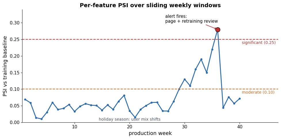
PSI over weekly production windows: values hover low for months, cross the moderate threshold, then breach the significant threshold where an alarm marker fires

Figure 1: A drift monitor in action: per-window PSI against the training baseline crosses the moderate band (0.1) and then the significant band (0.25), which is where alerting and retraining triggers fire.

Design details separate a working monitor from alert fatigue. Thresholds must account for sample size (small windows inflate every distance metric), per-feature tests need multiplicity control or aggregation, and the window length trades detection latency against statistical power. When labels are delayed, record them when they land and backfill realized metrics so you can audit how well the label-free estimators tracked reality. Finally, every alert needs a playbook: distinguish a broken upstream pipeline (schema violations, sudden null spikes) from genuine distribution drift, because the fix for the former is a data engineer, not a retraining job.

Monitoring stack flow: live traffic feeds input statistics checks and output confidence checks, delayed labels feed realized metrics, all signals join a decision block that routes to investigate, retrain, or roll back

Figure 2: The layered monitoring stack: input-distribution checks, output/confidence checks, and delayed-label evaluation feed one decision layer that separates pipeline breakage from genuine drift and triggers the right response.

Mathematical Formulation:
$\mathrm{PSI} = \sum_{b=1}^{B} (a_b - e_b)\,\ln\frac{a_b}{e_b}$
$D_{KS} = \max_x \, |F_{ref}(x) - F_{cur}(x)|$

Where:

$a_b$ and $e_b$ are the fractions of the current (actual) and reference (expected) samples in bin $b$ ; rules of thumb: PSI above 0.1 indicates moderate drift, above 0.25 significant drift.
$F_{ref}, F_{cur}$ are the empirical CDFs of the baseline and current window; $D_{KS}$ is their maximum vertical gap (the statistic behind SageMaker’s linf distance checks).
Both are computed per feature per window and compared against thresholds tuned for window size and alert budget.

Layer	Signal	Catches	Blind To
Input Stats	PSI / KS per feature vs baseline	Covariate shift, schema breakage	Concept drift
Output Stats	Prediction mix, confidence histogram	Label shift, confidence collapse	Silent concept drift
Estimated Performance	CBPE from calibrated probabilities	Accuracy loss under covariate shift	Concept drift (by assumption)
Delayed Ground Truth	Realized metrics when labels land	Everything, eventually	Nothing, but late

August 11, 2026

ML0085 Covariate Label Concept Drift

What is the difference between covariate shift, label shift, and concept drift?

Answer

All three are ways the joint distribution P(X, Y) at serving time can differ from training time, and they differ in which factor moved. Covariate shift: the input distribution P(X) changes while the labeling rule P(Y|X) stays fixed (your users got older, but age still means the same thing for risk). Label shift: the class prior P(Y) changes while the class-conditional input P(X|Y) stays fixed (fraud rate doubles in a crisis, but fraud still looks the same). Concept drift: the labeling rule P(Y|X) itself changes (the definition of spam evolves), so the model’s boundary is simply wrong now. Detection and repair differ per type, which is why the taxonomy matters operationally.

(1) Covariate Shift: P(X) moves, P(Y|X) fixed; visible in input statistics alone, and importance reweighting (weighting training points by density ratio) is the classical correction.
(2) Label Shift: P(Y) moves, P(X|Y) fixed; invisible in per-feature input stats if classes look alike, but visible in the model’s output distribution, and corrected by reweighting with estimated new priors.
(3) Concept Drift: P(Y|X) moves; no input-only monitor can see it in general, so you need ground truth (delayed labels) or estimation methods, and the only real fix is retraining on the new concept.

Three panels: covariate shift moves the input cloud while the boundary stays; label shift changes class proportions; concept drift rotates the boundary itself

Figure 1: The three drift types: covariate shift relocates the inputs (boundary still valid), label shift reweights class frequencies, and concept drift moves the true boundary, which invalidates the model even if inputs look unchanged.

The operational asymmetry is the interview-worthy insight. Input-side monitors (feature histograms, PSI, KS tests) reliably catch covariate shift and obvious label shift, because those live in P(X) and in the output distribution. But a pure concept drift can leave every input statistic untouched while accuracy collapses, which is why production monitoring stacks pair input-drift detectors with performance estimation or delayed ground-truth evaluation. NannyML’s CBPE documentation states exactly this split: confidence-based performance estimation stays accurate under covariate shift but cannot detect concept drift without labels.

Mathematical Formulation:
$P(X, Y) = P(Y \mid X)\,P(X) = P(X \mid Y)\,P(Y)$

Where:

$X$ is the input and $Y$ the target; the joint can be factorized in two directions.
Covariate shift: $P_{tr}(X) \neq P_{te}(X)$ while $P(Y \mid X)$ is unchanged.
Label shift: $P_{tr}(Y) \neq P_{te}(Y)$ while $P(X \mid Y)$ is unchanged; concept drift: $P(Y \mid X)$ itself changes (subscripts tr/te denote training vs serving).

Type	What Changes	Example	Detection Signal
Covariate Shift	P(X); boundary P(Y\|X) intact	User base ages; medical device sees older patients	Input stats (PSI/KS per feature)
Label Shift	P(Y); class appearance P(X\|Y) intact	Fraud rate spikes during a holiday season	Output/prediction distribution shift
Concept Drift	P(Y\|X); the rule itself moves	Spammers change tactics; same features, new meaning	Delayed labels; invisible to input-only monitors

August 11, 2026

ML0084 When Ensembles Fail

When can an ensemble of models perform worse than its best individual member?

Answer

Ensembles win through diversity, not through headcount. The ambiguity decomposition makes this exact: the ensemble’s error equals the average member error minus the average member disagreement, so combining helps only to the extent that members err on different examples. When errors are highly correlated, averaging or voting adds nothing and can dilute a genuinely better member. Stacked ensembles add a second failure surface: a meta-learner trained on too little or leaked validation data overfits the members’ quirks. And in production, the extra accuracy may not survive contact with engineering constraints, which is why Netflix never deployed the million-dollar Grand Prize ensemble.

(1) Diversity Is the Mechanism: majority voting only helps when member mistakes are at least partially independent; perfectly correlated members vote identically, and the ensemble is just the average member.
(2) Combination Failures: a strong model blended with weak-but-confident ones, or a stacking meta-learner fit on a tiny validation slice, can land below the best member; out-of-fold predictions and held-out weight tuning are the standard guards.
(3) Production Lesson (Netflix): the 2009 Grand Prize ensemble blended hundreds of models for a 10% RMSE gain, but Netflix reported the incremental accuracy “did not seem to justify the engineering effort” and shipped only two of the simpler Progress-Prize algorithms instead.

Two bar panels: with independent errors the majority vote beats every individual classifier, with correlated errors the vote falls below the best individual

Figure 1: The diversity condition: with independent errors (left) majority vote exceeds every member; with correlated errors (right) the vote inherits the shared blind spot and can fall below the best single model.

Two subtler traps complete the picture. First, aggregation weights: an average is optimal only when members are comparably accurate and comparably calibrated; one badly calibrated but overconfident member can dominate a soft-vote average and drag it below the best member. Second, the objective mismatch: members tuned individually for accuracy may combine poorly if their errors concentrate on the same hard slice; deliberately trading a little individual accuracy for decorrelation (different feature views, architectures, or training objectives) is how production ensembles are actually designed.

Mathematical Formulation:
$E_{ens} = \bar{E} - \bar{A}$
$\bar{A} = \frac{1}{M}\sum_{m=1}^{M} \mathrm{E}_x\left[ (f_m(x) - \bar{f}(x))^2 \right]$

Where:

$E_{ens}$ is the squared error of the average prediction $\bar{f}$ , and $\bar{E}$ is the mean of the members’ individual squared errors.
$\bar{A}$ is the ambiguity: the average squared disagreement of each member $f_m$ from the ensemble mean, i.e. the diversity dividend.
The ensemble beats the average member exactly by $\bar{A}$ ; if all members make identical errors then $\bar{A} = 0$ and ensembling gains nothing (Krogh-Vedelsby decomposition).

Failure Mode	Mechanism	Guard
Correlated Errors	Same architecture, features, and data produce shared blind spots	Diversify feature views, model families, training objectives
Overfit Stacking	Meta-learner trained on in-sample or tiny validation predictions	Out-of-fold predictions; simple meta-model (logistic, weighted mean)
Miscalibrated Member	Overconfident weak model dominates the soft vote	Calibrate members before averaging; weight by validation skill
Engineering Cost	Hundreds of members multiply latency, memory, and failure surface	Netflix lesson: ship the simple models that capture most of the gain

August 11, 2026