Category: Easy

DL0025 Attention Mechanism
Please explain the concept of “Attention Mechanism.”
Answer
The attention mechanism lets a model dynamically focus on the most relevant parts of the input when producing each output, instead of compressing the entire input into a single fixed-size context vector. For every output element, attention computes a weighted sum over input representations, where the weights (produced by a similarity score and a softmax) express how much each input element matters for that output. This solved the information bottleneck of early sequence-to-sequence models and is the core operation of Transformers.
(1) Query (Q): What the current output position is “looking for”: the element being processed.
(2) Key (K): An index of what each input position offers; queries are compared against keys to get similarity scores.
(3) Value (V): The actual content retrieved; scores are softmax-normalized into weights that blend the values into the output.

Figure 1: Attention weights are a probability distribution over inputs: here “machine” and “learning” absorb 72% of the weight for a topic-focused query.
Mathematical Formulation (Scaled Dot-Product Attention):
$\mathrm{Attention}(Q, K, V) = \mathrm{softmax}\left(\frac{QK^{\top}}{\sqrt{d_k}}\right) V$
Where:
$Q, K, V$ are the query, key, and value matrices, linear projections of the token embeddings.
$QK^{\top}$ holds the raw dot-product similarity scores between every query-key pair.
$\sqrt{d_k}$ scales the scores (key dimension $d_k$ ) to keep softmax out of its saturated, tiny-gradient region; softmax normalizes each row into weights summing to 1.
Login to view more content
July 20, 2025
DL0022 CNN Architecture
Describe the typical architecture of a CNN.
Answer
A typical Convolutional Neural Network chains together a small set of repeating building blocks: the raw input passes through stacked convolution + activation layers that extract local features, interleaved with pooling layers that halve the spatial resolution, after which the feature maps are flattened (or globally pooled) and fed into fully connected layers ending in a softmax output for classification. Regularizers such as dropout and batch normalization are commonly inserted along the way.
(1) Feature Extraction Front-End: Repeated conv → ReLU → pool blocks build hierarchical features while shrinking spatial size and growing channels.
(2) Classification Head: Flattened features (or a GAP vector) feed fully connected layers that combine features into class scores.
(3) Output Layer: Softmax for multi-class, sigmoid for binary/multi-label; optional dropout, batch norm, and skip connections stabilize training.

Figure 1: The canonical pipeline: spatial size shrinks (224 → 112 → 56) while channels grow (3 → 32 → 64), then a flatten + FC head classifies. Note the 200,704 values hitting the FC layer.
Mathematical Formulation:
$W_{out} = \left\lfloor \frac{W_{in} - k + 2p}{s} \right\rfloor + 1$
$P(y = i \mid z) = \frac{e^{z_i}}{\sum_{j=1}^{K} e^{z_j}}$
Where:
$W_{in}, W_{out}$ are the input and output spatial sizes of a conv or pool layer; $k$ is the kernel size, $p$ the padding, $s$ the stride.
$z_i$ is the logit for class $i$ ; $K$ is the number of classes; the softmax converts logits into a probability distribution.
Modern Variant: GAP Head: Many modern CNNs (ResNet, MobileNet) replace the flatten + large FC head with Global Average Pooling, which averages each feature map to a single number before a small classifier. This slashes parameters, removes the fixed-input constraint, and reduces overfitting.

Figure 2: Swapping flatten for GAP shrinks the classifier input from 200,704 to 64 values, millions fewer parameters in the head.
Login to view more content
May 31, 2025
DL0021 Feature Map
What is the feature map in Convolutional Neural Networks?
Answer
A feature map is the output produced when one convolutional filter slides across its input: a 2D grid of activations whose values encode where and how strongly a specific pattern (an edge orientation, texture, or object part) appears at each spatial location. A convolutional layer applies many filters in parallel, so its output is a stack of feature maps, one per filter, forming the layer’s channels.
(1) Output of One Filter: Each feature map is generated by a single filter convolving over the input; the layer output stacks one map per filter, so 64 filters produce 64 channels.
(2) Location and Strength: A high activation at position (i, j) means the filter’s pattern (e.g., a vertical edge or a corner) is strongly present around that location.
(3) Evolving Semantics with Depth: Early maps respond to edges and textures, middle maps to parts and shapes, and deep maps to whole objects with class-specific meaning.

Figure 1: Three filters applied to the same input produce three different feature maps; each lights up where its own pattern (vertical, horizontal, or any edge) appears.
Mathematical Formulation:
$y^{(c)}_{ij} = \sum_{a=1}^{k}\sum_{b=1}^{k}\sum_{d=1}^{C_{in}} w^{(c)}_{abd}\, x_{i+a,\, j+b,\, d} + b_c$
$\text{output shape} = (H_{out},\ W_{out},\ C_{out}), \quad C_{out} = \text{number of filters}$
Where:
$y^{(c)}_{ij}$ is the activation of feature map $c$ at spatial position $(i, j)$ .
$w^{(c)}_{abd}$ are the weights of filter $c$ of size $k \times k \times C_{in}$ ; $b_c$ is its bias.
$x_{i+a,\, j+b,\, d}$ is the input activation; $C_{in}$ and $C_{out}$ are the input and output channel counts.
Hierarchical Representation: As activations flow deeper, each new feature map is computed from the previous layer’s maps, so neurons see progressively larger receptive fields and combine simpler patterns into richer ones, the foundation of a CNN’s representational power.

Figure 2: Depth turns fine edges into parts and finally into an object-level representation. Resolution drops while semantic content rises.
Login to view more content
May 31, 2025
DL0020 CNN Parameter Sharing
How do Convolutional Neural Networks achieve parameter sharing? Why is it beneficial?
Answer
CNNs share parameters by applying the same convolutional filter at every spatial location: a small kernel of learnable weights slides across the input, and its weights are reused to compute each output activation. This weight reuse means the network learns location-independent features with far fewer parameters than a fully connected layer, which improves generalization and compute efficiency.
How Sharing Works:
(1) Convolutional Filter: A small matrix of learnable weights (e.g., $3 \times 3$ ) is defined per channel pair.
(2) Sliding Window: The filter moves across the whole input feature map, position by position.
(3) Weight Reuse: The identical weights are used at every position, so one filter detects its feature anywhere in the image.

Figure 1: The same 9 weights produce activations at position A and position B. No new parameters are added as the input grows.
Why It Is Beneficial:
(1) Reduced Parameters: A filter has $k \times k \times C_{in}$ weights regardless of input resolution, versus one weight per (input, output) pair in an FC layer.
(2) Translation Equivariance: A feature detected at one location is detected at any location; shifting the input shifts the output correspondingly.
(3) Improved Generalization: Fewer parameters means less overfitting, especially on limited data.
(4) Computational Efficiency: Fewer parameters mean fewer multiply-accumulates in both forward and backward passes, enabling deployment on resource-limited devices.

Figure 2: Translation equivariance in action: shifting the input shifts the convolution output by the same amount, because the same shared filter processes every position.
How Big Is the Saving? Sharing decouples the parameter count from the input resolution: growing the image grows the compute, not the weights. The contrast with a fully connected layer on the same input is dramatic.

Figure 3: Flattening a $32 \times 32 \times 3$ image into 100 FC units needs ~307k parameters; a shared $3 \times 3$ convolution with 64 filters needs ~1.8k, roughly 170x fewer.
Mathematical Formulation:
$y_{ijc} = \sum_{a=1}^{k}\sum_{b=1}^{k}\sum_{d=1}^{C_{in}} w_{abdc}\, x_{i+a,\, j+b,\, d} + b_c$
$P_{conv} = k^2 \cdot C_{in} \cdot C_{out} + C_{out}$
Where:
$y_{ijc}$ is the output activation at spatial position $(i, j)$ of channel $c$ ; the same $w$ is used for every $(i, j)$ : that reuse is parameter sharing.
$w_{abdc}$ is the filter weight at kernel offset $(a, b)$ connecting input channel $d$ to output channel $c$ ; $b_c$ is the per-output-channel bias.
$P_{conv}$ is the layer’s parameter count, independent of the input’s spatial size $H \times W$ .
Login to view more content
May 30, 2025
DL0017 Reproducibility
How do you ensure the reproducibility of deep learning experiments?
Answer
Reproducibility means a rerun of your experiment, by you or by someone else, produces the same results. Because deep learning pipelines are full of hidden randomness (weight initialization, data shuffling, dropout, GPU nondeterminism), achieving it requires controlling randomness with fixed seeds and deterministic operations, versioning code and configurations, pinning the software environment, fixing the dataset, and logging everything about each run.
(1) Seed Control and Deterministic Operations: Fix random seeds for Python, NumPy, and your framework (PyTorch/TensorFlow), and enable deterministic algorithms while disabling autotuners that pick nondeterministic kernels.
(2) Code and Configuration Versioning: Track code in Git and store every hyperparameter in versioned config files (YAML/JSON), so a run maps to an exact commit plus config.
(3) Environment and Dependency Control: Pin library versions (requirements.txt, Conda) or containerize with Docker, recording CUDA/cuDNN and hardware details.
(4) Dataset Management: Fix train/validation/test splits, document preprocessing, and use versioned datasets (e.g., DVC) so data never silently changes.
(5) Logging and Experiment Tracking: Record seeds, configs, metrics, and artifacts for every run with tools like MLflow or Weights & Biases.
What Failure Looks Like: Without seed control, two runs of identical code and data can trace visibly different accuracy curves (sometimes differing by a point or more at convergence), making results impossible to validate or compare.

Figure 1: Same code, same data, different curves: unseeded randomness alone is enough to make experiments non-reproducible.
A Practical Pipeline: Treat reproducibility as a chain: each link below removes one source of variability, and the result is reproducible only if every link holds.

Figure 2: Identical results require identical code + environment + data + seeds. A break in any link breaks the chain.
Mathematical Formulation:
$m = F(\text{code},\ \text{config},\ \text{env},\ \text{data},\ \text{seed})$
$\text{reproducible} \iff \forall\, i, j:\ m_i = m_j$
Where:
$F$ is the full experiment pipeline viewed as a function of its five inputs; $m$ is the resulting metric set (accuracy, loss curves).
$m_i, m_j$ are metrics from any two reruns; reproducibility demands zero variance across runs, which holds only when all five inputs are fixed.
Login to view more content
May 29, 2025
DL0016 Learning Rate Warmup
What is learning rate warmup, and why does it help stabilize the early steps of deep network training?
Answer
Learning rate warmup starts training with a very small learning rate and increases it gradually (usually linearly) to the target peak over the first few hundred or thousand steps, after which the normal schedule (e.g., cosine decay) takes over. Its purpose is to stabilize early training: at initialization the model’s gradients are noisy and poorly conditioned, so immediately applying the full learning rate can cause loss spikes, divergence, or permanent damage to early layers.
(1) Stabilizes Early Updates: Random initializations produce unreliable gradient estimates; small early steps prevent destructive weight changes before the model finds its footing.
(2) Protects Adaptive Optimizers: With Adam, second-moment estimates are cold at step zero and can amplify the first updates; warmup bridges this biased-estimate phase.
(3) Enables Higher Peak Rates: Deep networks and Transformers tolerate (and benefit from) a higher peak learning rate once representations have settled, which warmup makes reachable without instability.

Figure 1: A typical schedule: linear warmup for 200 steps to the 0.10 peak, then cosine decay to zero, the standard recipe behind models like BERT and GPT.
Mathematical Formulation:
$\eta_t = \eta_{max} \cdot \frac{t}{T_{warm}}, \quad t \leq T_{warm}$
$p = \frac{t - T_{warm}}{T - T_{warm}}$
$\eta_t = \eta_{max} \cdot \tfrac{1}{2}\big(1 + \cos(\pi p)\big)$
Where:
$\eta_t$ is the learning rate at step $t$ ; $\eta_{max}$ is the target peak learning rate.
$T_{warm}$ is the warmup length in steps (e.g., 200–10,000 depending on model and batch size).
$T$ is the total number of training steps; after warmup, the schedule shown is cosine decay.
$p \in [0, 1]$ is the post-warmup progress used by the third line, which applies once $T_{warm}$ steps have elapsed: $p = 0$ at the end of warmup and $p = 1$ at the final step, so $\eta_t$ decays from the peak to zero.
Why It Matters in Practice: Transformers are famously sensitive: without warmup their early loss can spike or diverge outright, while warmup yields a smooth descent; the effect is smaller but still useful in CNN training at very large batch sizes.

Figure 2: Without warmup the early loss can spike and diverge; warmup keeps the fragile first steps small until gradients become trustworthy.
Login to view more content
May 27, 2025
DL0011 Fully Connected Layer
Can you explain what a fully connected layer is?
Answer
A fully connected (FC) layer, also called a dense layer, is a layer in which every neuron connects to all neurons of the previous layer. It computes a weighted sum of its inputs, adds a bias, and applies an activation function, letting the network learn global combinations of features. FC layers typically appear at the end of a network, mapping extracted features to class scores.
(1) Dense Connectivity: With $n_{in}$ inputs and $n_{out}$ neurons, the layer holds $n_{in} \times n_{out}$ weights plus $n_{out}$ biases.
(2) Parameter Heavy: FC layers often dominate model size (e.g., flattening a $7 \times 7 \times 512$ map into 1000 classes needs ~25M parameters), which raises overfitting risk.
(3) Loses Spatial Structure: Inputs must be flattened, discarding spatial layout; Global Average Pooling (GAP) is a parameter-free alternative.
Mathematical Formulation:
$y = \sigma(Wx + b)$
$\#\text{params} = (n_{in} + 1) \times n_{out}$
Where:
$x \in \mathbb{R}^{n_{in}}$ is the flattened input vector and $y \in \mathbb{R}^{n_{out}}$ is the output vector.
$W \in \mathbb{R}^{n_{out} \times n_{in}}$ is the weight matrix and $b \in \mathbb{R}^{n_{out}}$ is the bias vector.
$\sigma$ is a non-linear activation such as ReLU (or softmax at the classifier output).

Figure 1: In an FC layer, every input neuron connects to every output neuron; each output is $\sigma(\sum_j w_j x_j + b)$ .
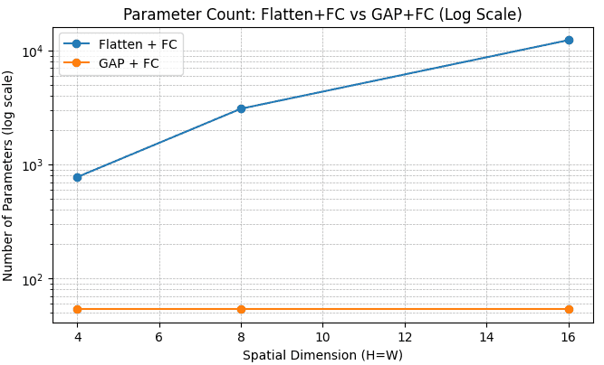
Flatten + FC vs GAP + FC: For a CNN head with $7 \times 7 \times 8$ feature maps and 6 classes, flattening feeds 392 values to the FC layer, while GAP feeds only 8, a 44× parameter reduction with less overfitting:
Approach FC Input Size FC Parameters Spatial Info
Flatten + FC $7 \times 7 \times 8 = 392$ $(392 + 1) \times 6 = 2358$ Discarded by flattening
GAP + FC $8$ (one per channel) $(8 + 1) \times 6 = 54$ Summarized per channel

Figure 2: GAP collapses each feature map to one value before the FC layer, cutting parameters from 2358 to 54 in this example.
Login to view more content
May 3, 2025

Approach	FC Input Size	FC Parameters	Spatial Info
Flatten + FC	$7 \times 7 \times 8 = 392$	$(392 + 1) \times 6 = 2358$	Discarded by flattening
GAP + FC	$8$ (one per channel)	$(8 + 1) \times 6 = 54$	Summarized per channel

DL0009 Pooling

Please compare max pooling and average pooling in deep learning, and explain in which scenarios you would prefer one over the other.

Answer

Max pooling selects the maximum value within each window of the feature map, keeping the strongest activation in every region. Average pooling computes the mean of all values in the window, producing a smoothed, holistic summary. Both downsample the feature map, but they preserve different information: max pooling keeps sharp, distinctive activations, while average pooling retains the overall activation distribution.

(1) Operation Difference: Max pooling takes the peak activation per window; average pooling takes the window mean: one is sharp and selective, the other smooth and inclusive.
(2) Information Retention: Max pooling may discard weaker features but ignores minor noisy activations; average pooling keeps more of the overall distribution but can average noise into the output.
(3) Typical Use Cases: Prefer max pooling for classification and object detection where feature presence matters; prefer average pooling for segmentation and Global Average Pooling (GAP) where a holistic summary matters.

Mathematical Formulation:
$n_{out} = \left\lfloor \frac{n_{in} - k}{s} \right\rfloor + 1$

Where:

$n_{out}$ and $n_{in}$ are the output and input spatial sizes (identical formula for max and average pooling).
$k$ is the pooling window size and $s$ is the stride (commonly $s = k$ ).

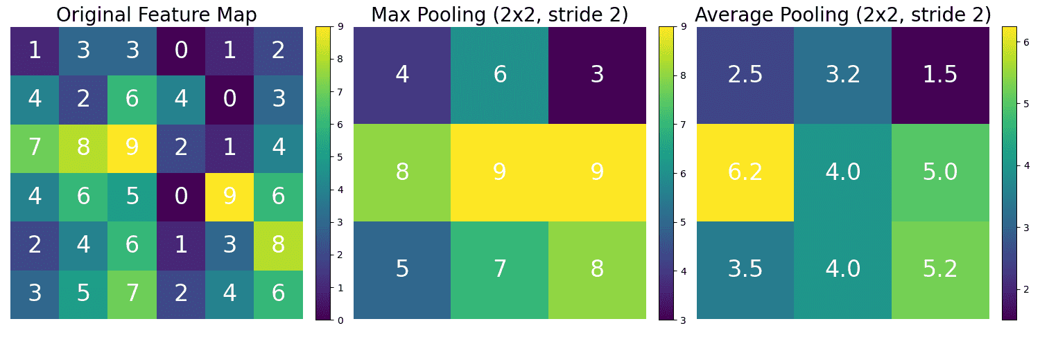
Side-by-side worked example of max pooling and average pooling applied to the same 4x4 input with 2x2 windows, producing different 2x2 outputs.

Figure 1: With 2×2 windows and stride 2, max pooling keeps each region’s peak value while average pooling smooths each region into its mean.

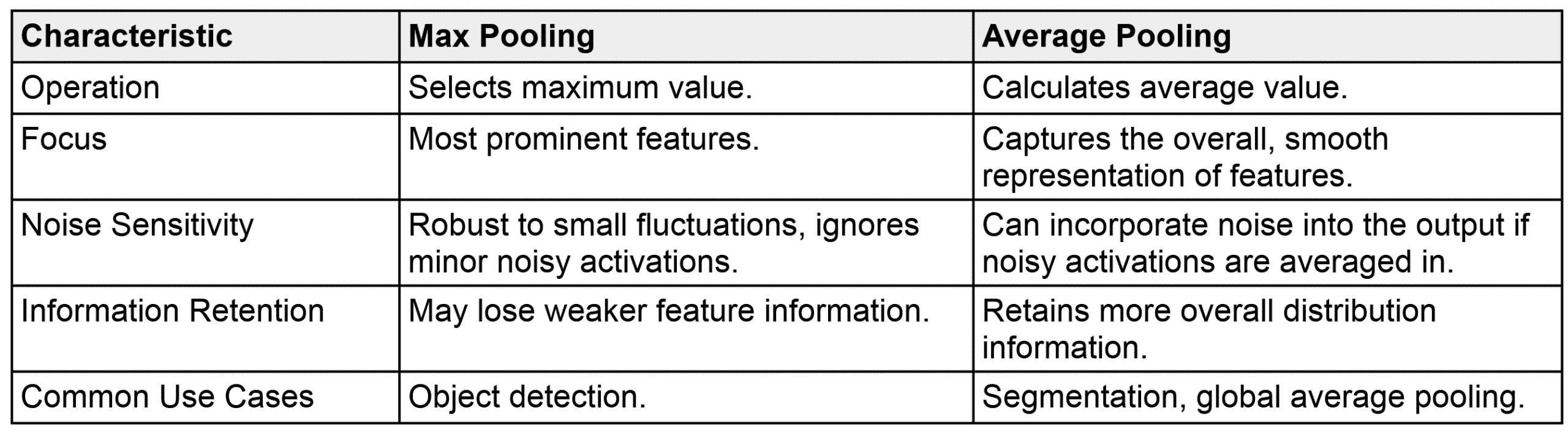
Max Pooling vs Average Pooling in Summary:

Characteristic	Max Pooling	Average Pooling
Operation	Selects maximum value	Calculates average value
Focus	Most prominent features	Overall, smooth representation of features
Noise Sensitivity	Robust to small fluctuations; ignores minor noisy activations	Can incorporate noise if noisy activations are averaged in
Information Retention	May lose weaker feature information	Retains more overall distribution information
Common Use Cases	Object detection, classification	Segmentation, global average pooling

When to Prefer Which: Choose max pooling when the presence of a feature matters more than its exact magnitude, as in detecting edges, textures, or objects. Choose average pooling when you need a balanced regional summary, e.g., aggregating context for segmentation or collapsing feature maps with GAP before the classifier.

Decision flow for choosing max pooling or average pooling based on whether sharp feature presence or a smooth holistic summary is needed.

Figure 2: Decision guide: sharp feature presence points to max pooling; a smooth holistic summary points to average pooling.

May 1, 2025

DL0008 Hyperparameter Tuning
What are the common strategies for hyperparameter tuning in deep learning?
Answer
Hyperparameter tuning optimizes the configuration settings that control the learning process, such as learning rate, batch size, and architecture choices. Because each evaluation requires training a model, the goal is to find strong configurations with as few trials as possible, which makes sample-efficient search strategies essential.
(1) Manual/Heuristic Search: Start with values from prior work or common practice and iteratively adjust based on validation performance.
(2) Grid Search: Exhaustively evaluate all combinations over a predefined discrete grid; simple but scales poorly with dimensionality.
(3) Random Search: Randomly sample values from predefined ranges; covers more distinct values per hyperparameter than grid search for the same budget.
(4) Bayesian Optimization: Use a probabilistic surrogate model to intelligently suggest the next configuration, balancing exploration vs exploitation.

Figure 1: With 9 trials, grid search tests only 3 distinct learning rates, while random search covers 9 distinct values, which matters when one hyperparameter is much more important than the others.
Mathematical Formulation:
$EI(x) = \mathbb{E}\left[\max\left(f(x) - f(x^*),\ 0\right)\right]$
$x_{next} = \arg\max_{x}\ \alpha(x;\ \mathcal{D})$
Where:
$EI(x)$ is the Expected Improvement acquisition function: the expected amount by which $f(x)$ exceeds the best observed score $f(x^*)$ (for maximization).
$\alpha(x;\mathcal{D})$ is the acquisition function (e.g., EI or UCB) computed from the surrogate model fitted on past trials $\mathcal{D}$ ; maximizing it picks the next configuration to evaluate.

Figure 2: Bayesian optimization iterates: fit a surrogate model, pick the next point via an acquisition function, evaluate it, and update the model, repeating until the trial budget is spent.
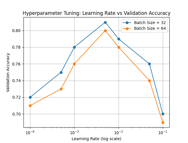
Hyperparameter Interactions: Validation accuracy is non-monotonic in learning rate, and the optimum shifts with batch size. That is one reason joint search beats tuning one hyperparameter at a time.

Figure 3: Accuracy peaks in the same best lr region for both batch sizes, but the curves differ: hyperparameters interact and should be tuned jointly.
Login to view more content
April 30, 2025
DL0007 Batch Norm
Why use batch normalization in deep learning training?
Answer
Batch normalization stabilizes and accelerates training by normalizing each layer’s inputs across the mini-batch: subtract the batch mean and divide by the batch standard deviation. After normalization, a learnable scale $\gamma$ and shift $\beta$ let the network recover the identity transformation if needed. BN is applied after the linear transform (e.g., the convolution) and before the activation (e.g., ReLU).
(1) Stabilizes Learning: Reduces internal covariate shift, making training less sensitive to initialization and hyperparameter choices.
(2) Enables Higher Learning Rates: Larger learning rates can be used without instability, leading to faster convergence.
(3) Improves Generalization: Normalizing per mini-batch introduces noise into activations, preventing over-reliance on specific batches and acting as a mild regularizer.

Figure 1: Each feature channel is normalized using its mini-batch statistics, then rescaled by learnable $\gamma$ and $\beta$ .
Mathematical Formulation:
$BN(x_i) = \gamma \left( \frac{x_i - \mu_B}{\sqrt{\sigma_B^2 + \epsilon}} \right) + \beta$
Where:
$x_i$ is an individual feature value in the batch.
$\mu_B$ and $\sigma_B^2$ are the mean and variance of that feature across the current mini-batch.
$\epsilon$ is a small constant (e.g., $10^{-5}$ ) added for numerical stability.
$\gamma$ and $\beta$ are learnable scaling and shifting parameters.

Figure 2: Training computes per-batch statistics and updates running averages; inference uses the frozen running averages, producing deterministic outputs.
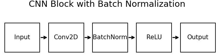
Placement in a CNN Block: BN sits between the linear transform and the non-linearity: Conv2D → BatchNorm → ReLU.

Figure 3: In a standard CNN block, BatchNorm normalizes the convolution output before the activation function.
Login to view more content
April 30, 2025