Interview for Machine Learning

Category: Easy

DL0049 Weight Init
Why is “weight initialization” important in deep neural networks?
Answer
Weight initialization is crucial for stabilizing activations and gradients, enabling deep neural networks to train efficiently and converge faster without numerical instability.
(1) Prevents vanishing/exploding gradients: Proper initialization keeps activations and gradients within reasonable ranges during forward and backward passes
(2) Ensures faster convergence: Good initialization allows the optimizer to reach a good solution more quickly.
(3) Breaks symmetry: Different initial weights ensure neurons learn unique features rather than identical outputs.

Xavier Initialization is used for activations like Sigmoid or Tanh:
Xavier aims to keep the variance of activations consistent across layers for symmetric activations (tanh/sigmoid).
$W \sim \mathcal{N}\left(0, \frac{1}{n_{\text{in}} + n_{\text{out}}}\right)$
or (uniform version):
$W \sim \mathcal{U}\left(-\sqrt{\frac{6}{n_{\text{in}} + n_{\text{out}}}}, \sqrt{\frac{6}{n_{\text{in}} + n_{\text{out}}}}\right)$
Where:
$n_{\text{in}}$ = number of input units
$n_{\text{out}}$ = number of output units
$\mathcal{N}(\mu, \sigma^2)$ means weights are sampled from a normal (Gaussian) distribution with mean $\mu$ and variance $\sigma^2$ .
$\mathcal{U}(a, b)$ means weights are sampled from a uniform distribution in the range $[a, b]$ .
He Initialization is used for activations like ReLU or Leaky ReLU:
He initialization scales up the variance for ReLU, since half of its outputs are zero, preventing vanishing activations.
$W \sim \mathcal{N}\left(0, \frac{2}{n_{\text{in}}}\right)$
or (uniform version):
$W \sim \mathcal{U}\left(-\sqrt{\frac{6}{n_{\text{in}}}}, \sqrt{\frac{6}{n_{\text{in}}}}\right)$
Where:
$n_{\text{in}}$ = number of input units
He initialization is recommended for ReLU networks as shown in the plot below.
Login to view more content
October 28, 2025
DL0048 Adam Optimizer
Can you explain how the Adam optimizer works?
Answer
The Adam (Adaptive Moment Estimation) optimizer is a powerful algorithm for training deep learning models, combining the principles of Momentum and RMSprop to compute adaptive learning rates for each parameter.
Adam updates following the steps below:
(1) First Moment Calculation(Mean/Momentum)
It computes an exponentially decaying average of past gradients, which is the estimate of the first moment (mean) of the gradient. This introduces a momentum effect to smooth out the updates.
$m_t = \beta_1 m_{t-1} + (1 - \beta_1) g_t$
Where:
$m_t$ is the 1st moment (mean of gradients).
$g_t$ is the gradient at step $t$ .
$\beta_1$ controls momentum (default: 0.9).
(2) Second Moment Calculation (Variance)
Adam also computes an exponentially decaying average of past squared gradients, which is the estimate of the second moment (uncentered variance) of the gradient. This provides a measure of the scale (magnitude) of the gradients.
$v_t = \beta_2 v_{t-1} + (1 - \beta_2) g_t^2$
Where:
$v_t$ is the 2nd moment (variance of gradients).
$\beta_2$ controls smoothing of squared gradients (default: 0.999).
(3) Bias Correction
Since $m_t$ and $v_t$ are initialized as zero vectors, they are biased towards zero, especially during the initial steps. Adam applies bias correction to these estimates.
$\hat{m}_t = \frac{m_t}{1 - \beta_1^t}$
$\hat{v}_t = \frac{v_t}{1 - \beta_2^t}$
Where
$\hat{m}_t$ is the bias-corrected 1st moment.
$\hat{v}_t$ is the bias-corrected 2nd moment.
$\beta_1^t$ , $\beta_2^t$ are the exponential decay raised to step $t$ , correcting bias from initialization.
(4) Parameter Update
The final parameter update scales the bias-corrected first moment ( $m_t$ ) by the overall learning rate ( $\alpha$ ) and divides by the square root of the bias-corrected second moment ( $v_t$ ).
$\theta_t = \theta_{t-1} - \alpha \frac{\hat{m}_t}{\sqrt{\hat{v}_t} + \epsilon}$
Where:
$\theta_t$ are model parameters.
$\alpha$ is the learning rate.
$\epsilon$ prevents division by zero.
The plot below shows how the Adam optimizer efficiently moves from the starting point to the minimum of the quadratic bowl, taking adaptive steps that quickly converge to the origin.
Login to view more content
October 27, 2025
DL0046 Focal Loss
What is focal loss, and why does it help with class imbalance?
Answer
Focal loss augments cross-entropy with a modulating term $(1 - p_t)^\gamma$ and an optional balancing weight $\alpha_t$ to suppress gradients from easy, majority-class examples and amplify learning from hard or minority-class examples, improving performance in severe class-imbalance settings when hyperparameters are properly tuned.
(1) Focal loss formula:
$\text{FocalLoss}(p_t) = -\alpha_t (1 - p_t)^\gamma \log(p_t)$
Where:
$p_t$ is the model probability for the ground-truth class;
$\gamma \ge 0$ is the focusing parameter that down-weights easy examples;
$\alpha_t \in (0,1)$ is an optional class-balancing weight for class t.
(2) Modulation: The factor $(1 - p_t)^\gamma$ reduces loss from well-classified (high-confidence) examples, concentrating gradients on hard / low-confidence examples.

(3) Class imbalance effect:
In cross-entropy, abundant, easy negatives still produce a large total gradient, dominating learning.
Focal loss down-weights those contributions, ensuring rare/difficult samples have a stronger influence.
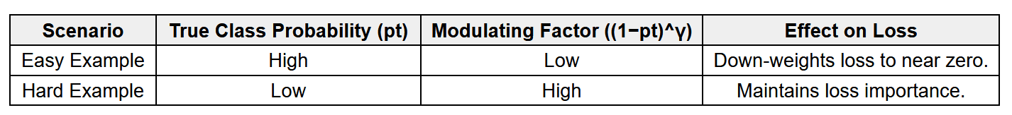
The plot below shows cross-entropy and focal-loss curves for several $\gamma$ values and an example $\alpha$ .
Login to view more content
October 27, 2025
DL0043 KV Cache
What is KV Cache in transformers, and why is it useful during inference?
Answer
The KV Cache in transformers optimizes inference by storing and reusing key and value vectors from the attention mechanism, avoiding redundant computations for previous tokens in a sequence. This is particularly useful in autoregressive models, where each new token requires attention over all prior tokens. By caching K and V vectors, the model only computes the query for the new token and retrieves cached K and V for earlier tokens, improving speed at the cost of higher memory usage.
The attention mechanism, optimized by KV Cache, is:
$\mathrm{Attention}(Q_t, K_{1:t}, V_{1:t}) = \mathrm{Softmax}\left(\frac{Q_t K_{1:t}^\top}{\sqrt{d_k}}\right) V_{1:t}$
Where:
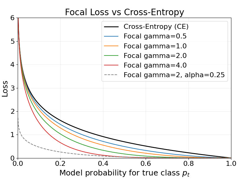
$Q_t$ = query of the current token t.
$K_{1:t}, V_{1:t}$ = cached keys and values for all tokens up to t.
$d_k$ = key dimension.
The figure below explains the KV cache in autoregressive transformers.
Login to view more content
September 14, 2025
DL0040 Attention Mask
What is the role of masking in attention?
Answer
Masking is a critical technique in transformer attention mechanisms that controls which parts of the input sequence the model is allowed to focus on.
(1) Leakage prevention: Blocks access to future tokens in autoregressive decoding to preserve causality.
(2) Padding handling: Excludes pad positions so they don’t absorb probability mass or distort context.
(3) Structured constraint: Enforces task rules (e.g., graph neighborhoods, spans, or blocked regions).
Core equation with mask:
$\text{Attn}(Q,K,V,M)=\text{Softmax}\left(\frac{QK^\top}{\sqrt{d_k}}+M\right)V$
Where:
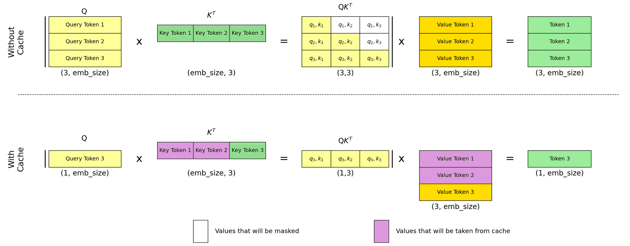
$Q$ query matrix.
$K$ key matrix.
$V$ value matrix.
$d_k$ key dimensionality (for scaling).
$M$ mask matrix with 0 for allowed positions and large negative values (e.g., −∞) for disallowed positions.
The figure below shows three side-by-side heatmaps: a padding mask that disallows attending to padding tokens, a causal mask that enforces autoregressive decoding, and a structured mask that enforces local neighborhood constraint.
Login to view more content
August 31, 2025
DL0038 Transformer Activation
Which activation functions do transformer models use?
Answer
Transformers mainly use GELU/ReLU in the feed-forward layers to introduce non-linearity and Softmax in attention to produce normalized attention weights. GELU is preferred for smoother gradient flow and better performance.
(1) Feed-Forward Network (FFN):
Uses ReLU or GELU as the non-linear activation.
GELU is more common in modern Transformers (like BERT, GPT).
Equation for GELU:
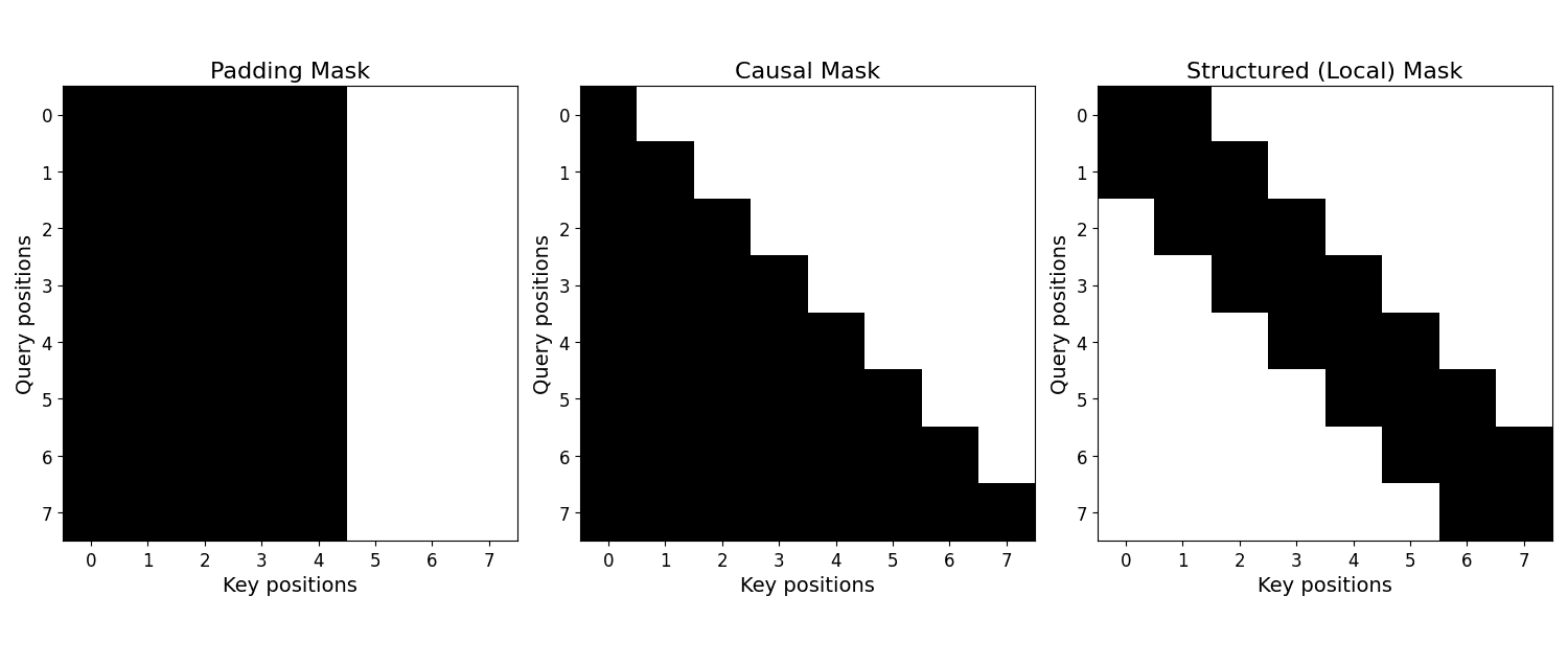
$\mbox{GELU}(x) = x \cdot \Phi(x) = x \cdot \frac{1}{2}\left[1 + \mbox{erf}\left(\frac{x}{\sqrt{2}}\right)\right]$
Where:
$x$ is the input,
$\Phi(x)$ is the Cumulative Distribution Function (CDF) of the standard Gaussian.
The figure below demonstrates the difference between ReLU and GELU.
(2) Attention Output:
Uses Softmax to convert attention scores into probabilities.
Equation for Softmax:
$\mbox{Softmax}(z_i) = \frac{e^{z_i}}{\sum_{j=1}^{K} e^{z_j}}$
Where:
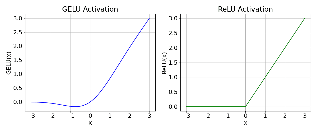
$z_i$ represents the raw attention score for the i-th token,
$K$ is the total number of tokens considered in attention.
Login to view more content
August 26, 2025
DL0036 Transformer Architecture II
What are the main differences between the encoder and decoder in a Transformer?
Answer
The encoder focuses on encoding input into rich representations via bidirectional self-attention, while the decoder leverages these for output generation through masked self-attention and cross-attention, ensuring autoregressive and context-aware predictions.
(1) Self‑Attention:
Encoder: Unmasked, attends to all positions in the input sequence.
Decoder: Masked, attends only to past positions to maintain causal order.
(2) Cross‑Attention:
Encoder: None.
Decoder: Present — attends to encoder outputs for context.
(3) Masking:
Encoder: No masking needed.
Decoder: Causal mask prevents looking ahead.
(4) Positional Encoding:
Encoder: Added to source embeddings.
Decoder: Added to target embeddings (shifted right during training).
(5) Function:
Encoder: Encodes the full source sequence into contextual representations.
Decoder: Generates the target sequence one token at a time using its own history and encoder context.
The figure below shows the encoder and the decoder in the Transformer.
Login to view more content
August 17, 2025
DL0035 Transformer Architecture
Describe the original Transformer encoder–decoder architecture.
Answer
The original Transformer model has an encoder-decoder architecture. The encoder processes the input sequence (e.g., a sentence) to create a contextual representation for each word. The decoder then uses this representation to generate the output sequence (e.g., the translated sentence), one word at a time. This entire process relies on attention mechanisms instead of recurrence.
Overall: Sequence-to-sequence encoder–decoder model with 6 encoder layers and 6 decoder layers [1].
Encoder layer:
(1) Multi-Head Self-Attention (all tokens attend to each other).
(2) Position-wise Feed-Forward Network (two linear layers + ReLU).
(3) Residual connection + LayerNorm after each sublayer.
Decoder layer:
(1) Masked Multi-Head Self-Attention (prevents seeing future tokens).
(2) Cross-Attention (queries from decoder, keys/values from encoder output).
(3) Position-wise Feed-Forward Network.
(4) Residual connection + LayerNorm after each sublayer.
Input representation: Inputs are represented as token embeddings summed with positional encodings to preserve sequence order, as the attention mechanism is permutation-invariant.
Output: The final decoder output passes through a linear projection layer, followed by softmax to produce probabilities over the target vocabulary for next-token prediction.
The figure below shows the architecture of the Transformer.

References:
[1] Vaswani, Ashish, et al. “Attention is all you need.” Advances in neural information processing systems 30 (2017).
Login to view more content
August 14, 2025
DL0034 Layer Norm
What is layer normalization, and why is it used in Transformers?
Answer
Layer Normalization is a technique that standardizes the inputs across the features for a single training example. Unlike Batch Normalization, which normalizes across the batch dimension, Layer Normalization computes the mean and variance for every single example independently to normalize its features.
(1) Normalization within a Sample: Layer Normalization (LN) calculates the mean and variance across all the features of a single data point (e.g., a single token’s embedding vector in a sequence). It then uses these statistics to normalize the features for that data point only.
(2) Batch Size Independence: Because it operates on individual examples, its calculations are independent of the batch size. This is a major advantage in models like Transformers that often process sequences of varying lengths, which can make batch statistics unstable.
(3) Stabilizes Training: By keeping the activations in each layer within a consistent range (mean of 0, standard deviation of 1), LN helps prevent the exploding or vanishing gradients problem. This leads to a smoother training process and faster convergence, especially in deep networks.
Layer Normalization Equation:
$\hat{x}_i = \frac{x_i - \mu}{\sigma + \epsilon} \cdot \gamma + \beta$
Where:
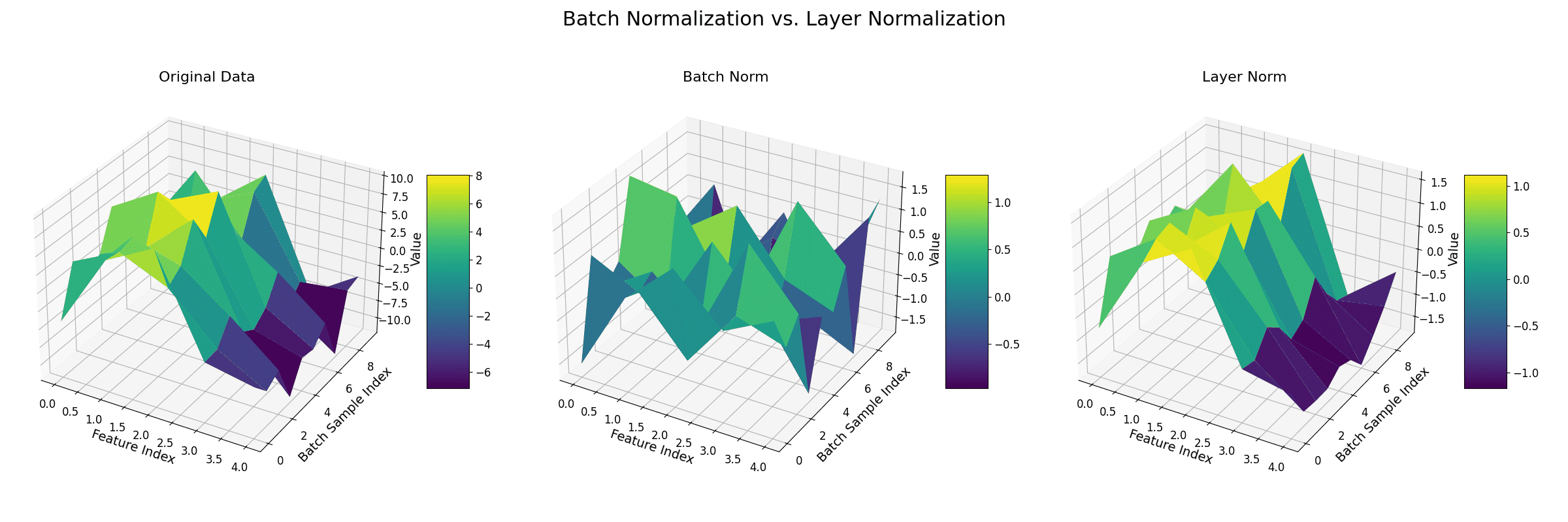
$x_i$ = input feature,
$\mu$ = mean of all features for the current sample,
$\sigma$ = standard deviation of all features,
$\epsilon$ = small constant for numerical stability,
$\gamma, \beta$ = learnable scale and shift parameters.
The figure below demonstrates the difference between batch normalization and layer normalization.
Login to view more content
August 14, 2025
DL0032 Transformer VS RNN
What makes Transformers more parallel-friendly than RNNs?
Answer
The fundamental difference lies in their architecture: RNNs sequentially process data, with each step depending on the output of the previous one. Transformers, on the other hand, utilize attention to examine all parts of the sequence simultaneously, enabling parallel processing. This parallelizability is a key reason for the Transformer’s superior performance on many tasks and its dominance in modern natural language processing.
(1) No Temporal Dependency: Transformers process all input tokens simultaneously, unlike RNNs, which depend on previous hidden states.
(2) Self-Attention is Fully Parallelizable: Attention scores are computed for all positions in a single pass.
(3) Optimized for GPUs: Matrix multiplications in Transformers leverage GPU cores better than the sequential loops in RNNs.
The figure below demonstrates the architectures of RNNs and Transformers.
Login to view more content
August 10, 2025