What makes Transformers more parallel-friendly than RNNs?
Answer
The fundamental difference lies in their architecture: RNNs sequentially process data, with each step depending on the output of the previous one. Transformers, on the other hand, utilize attention to examine all parts of the sequence simultaneously, enabling parallel processing. This parallelizability is a key reason for the Transformer’s superior performance on many tasks and its dominance in modern natural language processing.
(1) No Temporal Dependency: Transformers process all input tokens simultaneously, unlike RNNs, which depend on previous hidden states.
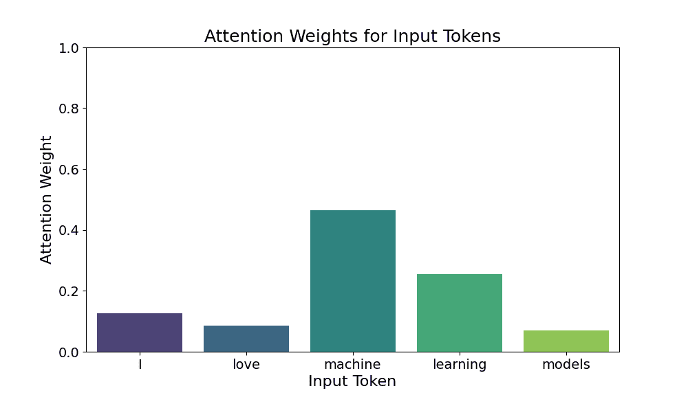
(2) Self-Attention is Fully Parallelizable: Attention scores are computed for all positions in a single pass.
(3) Optimized for GPUs: Matrix multiplications in Transformers leverage GPU cores better than the sequential loops in RNNs.
The figure below demonstrates the architectures of RNNs and Transformers.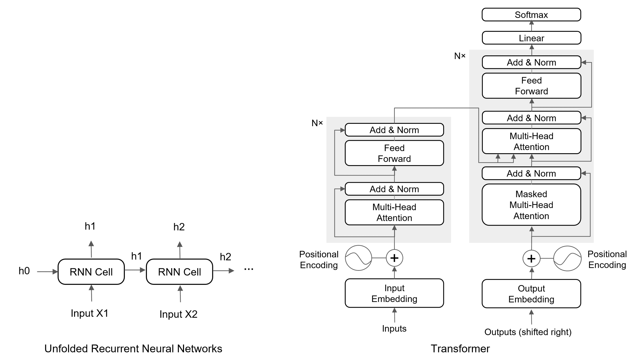

 — input vector for a token after the attention layer
 — trainable weight matrices
 — trainable bias vectors
 — ReLU activation (sometimes replaced by GELU)

 : token position in the sequence
 : dimension index
 : embedding dimension


 : Final output projection matrix that maps the concatenated attention outputs back to the original model dimension.
 : Number of attention heads.
 : Dimension of each head’s projected subspace.

 ,
,  , and
, and  represent query, key, and value matrices, respectively
 is the dimensionality of the key vectors

 : Matrices of queries, keys, and values.
 : Converts similarity scores to probabilities.